Exploration, Mapping and Scalar Field Estimation using a Swarm of Resource-Constrained Robots
Ragesh Kumar Ramachandran
Advisor : Dr Spring Berman
Autonomous Collective Systems Laboratory



Motivation
Development of robot platforms that can be deployed in swarms to perform tasks autonomously over large spatial and temporal scales.
Many potential applications for robotic swarms, including exploration, environmental monitoring, disaster response, search-and-rescue, mining, and intelligence-surveillance-reconnaissance, will require to operate in dynamic, uncertain and GPS denied environments
Despite these limitations, it may be necessary for the swarm to characterize its surroundings, for instance to map obstacles, payloads for transport, or hazardous areas to avoid.
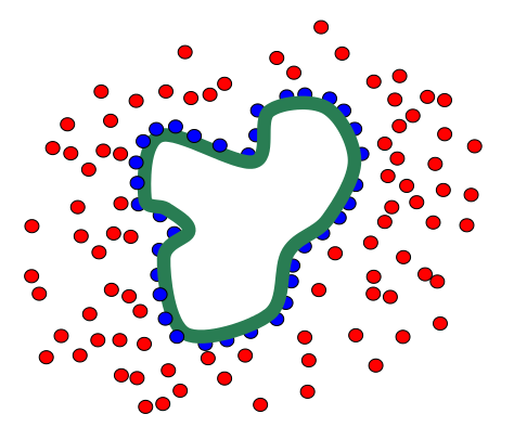
Our current research progress and future work focus on novel estimation and mapping strategies using robotic swarms in these types of applications.
Overview
An Advection-Diffusion-Reaction Based Approach to Mapping an Environmental Feature.
A Probabilistic Topological Approach to Quantifying Environmental Features.
A Probabilistic Approach to Constructing Topological Maps of an Environment.
Metric Map Construction using a Stochastic Robotic Swarm Leveraging Received Signal Strength.
Distributed mapping and information theoretic exploration.
Scalar Field Estimation by Large Networks with Partially Accessible Measurements.
Ongoing work
An Advection-Diffusion-Reaction Based Approach to Mapping an Environmental Feature*
*Ragesh K. Ramachandran, Karthik Elamvazhuthi, and Spring Berman. An optimal control approach to mapping GPS-denied environments using a stochastic robotic swarm. In Int’l. Symp. on Robotics Research (ISRR), 2015
Problem Statement
Mapping a single feature of interest using a robotic swarm without communication or localization capabilities.
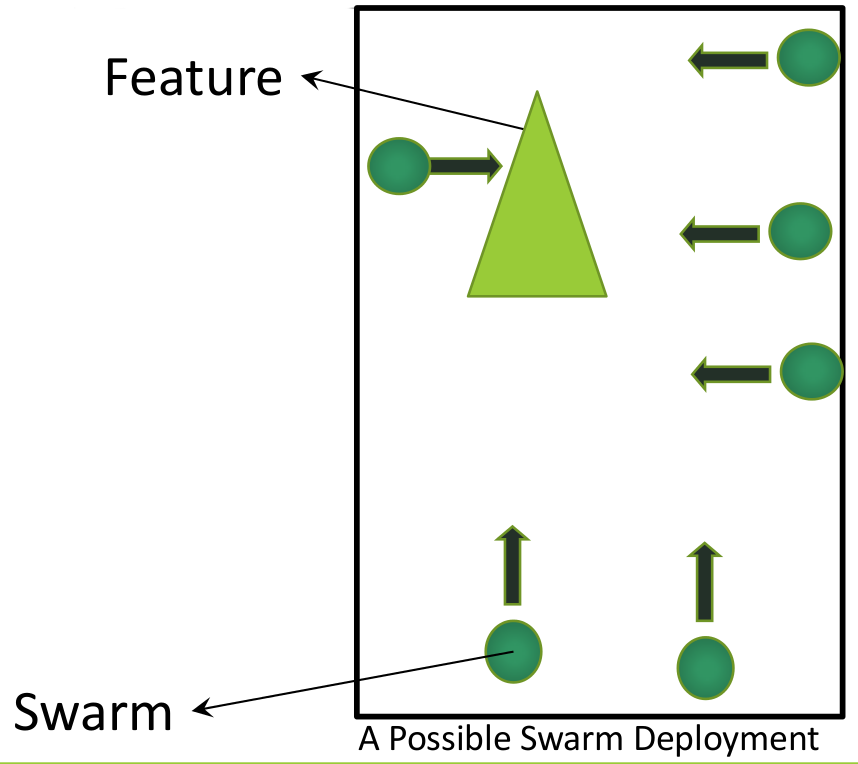
Robotic swarm models
Robotic swarms with stochastic behaviors.
Macroscopic abstraction using partial differential equations
Mapping formulated as an optimal control problem.
Related Work
The most common approach in robotics is SLAM and probabilistic mapping.
Mapping an environment using a robotic swarm is a relatively new area of research in the robotics.
In Dirafzoon et al.(2013)a robotic swarm is used to identify the topological features of an environment from information about the times at which robots encounter other robots and environmental features.
Microscopic Model
Robot State Changes (Chemical Reactions)

Robot Motion Model
$$\textbf{X}_i(t + \Delta t) = \textbf{X}_i(t) + (\sqrt{2D \Delta t}) \mathbf{Z}(t) + \textbf{v}(t) \Delta t$$
Microscopic Model Simulation
Macroscopic Model
No-flux Boundary Conditions : $\vec{n} \cdot (D\nabla u - \mathbf{v}(t)u) = 0 ~~~ on ~~\partial \Omega \times [0,T] $
Initial Condition : Gaussian density centered at a point $\mathbf{x}_0 \in \Omega$
u(x,t) := Active robot density, D := Diffusion coefficient, $\mathbf{v}(t)$ := Velocity field
k := Reaction rate constant, $K(\mathbf{x})$ := Feature Indicator Function (Map)
Optimal Control Problem
Objective Function
$$\underset{(\mathbf{u},K(\mathbf{x})) \in U^N \times \Theta_{ad}}{\min}\mathbf{J}(\mathbf{u},K) = \sum_{i = 1}^{N} W_i J_i(u_i) + \frac{\lambda}{2}\|K(\mathbf{x})\|^2_{L^2(\Omega)}$$ $$J_i(u_i) = \frac{1}{2}\left \| \int_{\Omega} u_i(\mathbf{x},t) d\mathbf{x} - g_i(t)\right \|_{L^2([0,T])}^2$$Admissible control inputs
$\Theta_{ad} = \{ K(\mathbf{x}) \in L^2(\Omega); ~K_{min} \leq K(\mathbf{x}) \leq K_{max} \}$With the macroscopic model as Constraint equations
Lagrangian Equation
The optimization problem is solved using a gradient descent approach
$$\mathcal{L}(\mathbf{u},\mathbf{p},K) = \mathbf{J}(\mathbf{u},K) + \sum_{i = 1}^{N} \langle p_i, \Psi_i(u_i,K) \rangle$$$\Psi_i(u_i,K)$ is the $i^{th}$ constraint and $p_i$ is the adjoint variable.
Gradient Equation
$$\mathbf{J}' = \sum_{i = 1}^{N} (\int_0^T(ku_ip_i)(\mathbf{x})dt) + \lambda K(\mathbf{x})$$
$p_i$ is computed by solving the adjoint equation.
Adjoint Equation
The equations are solved backwards
Simulation Results
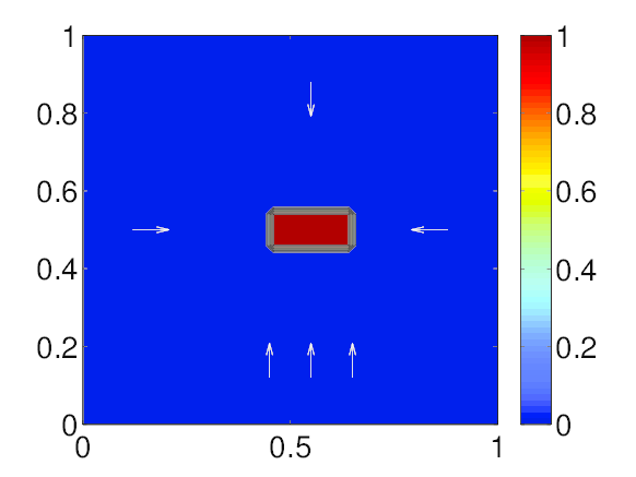
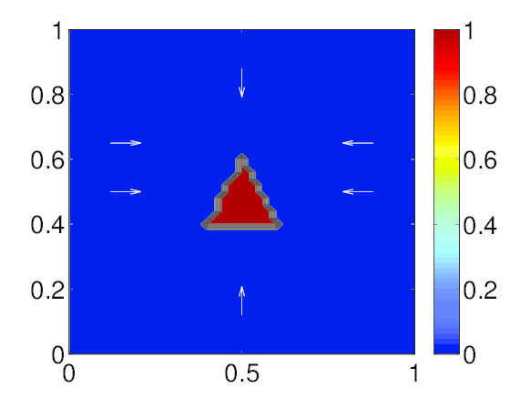
Actual map
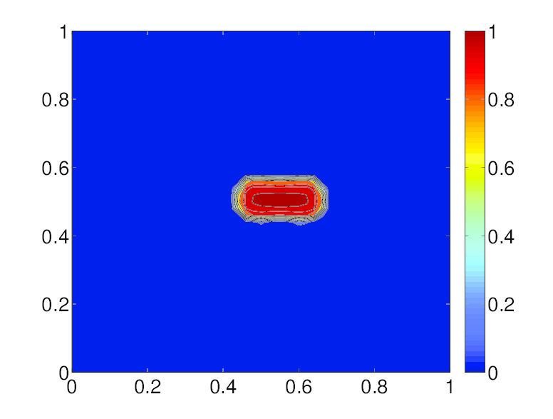
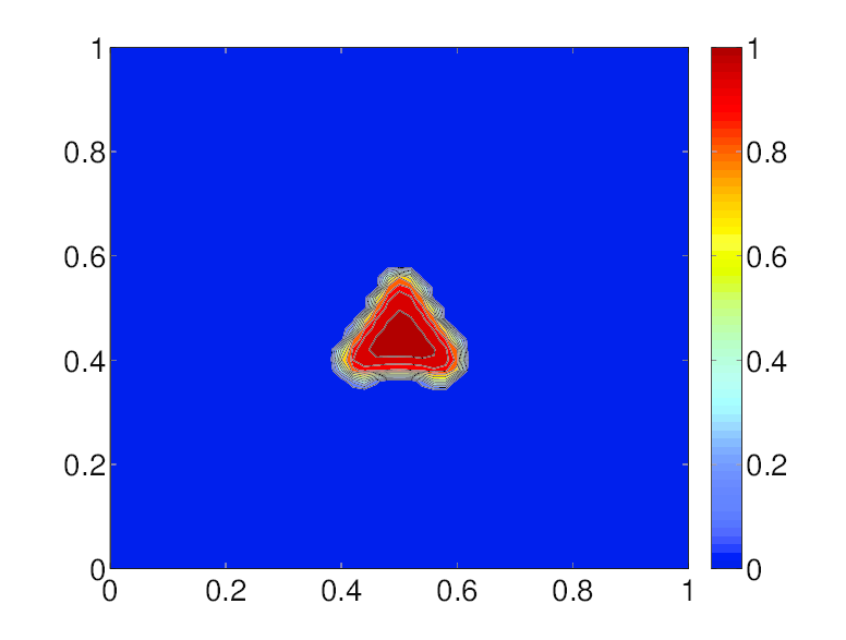
Estimated map

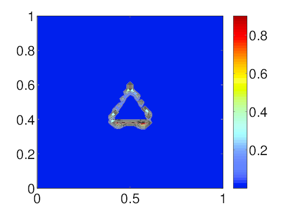
Absolute value of error
Simulation Results
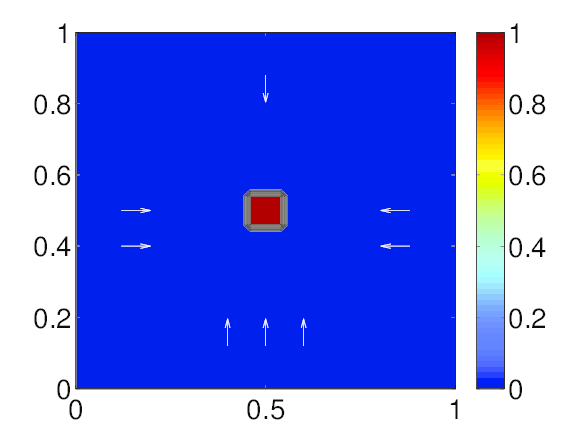
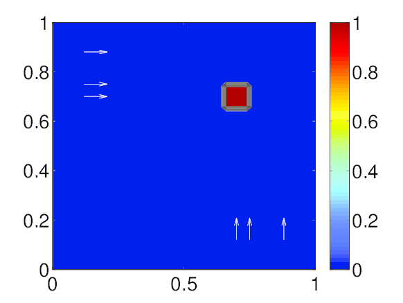
Actual map
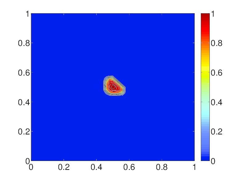
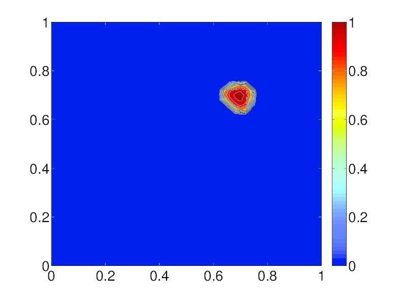
Estimated map
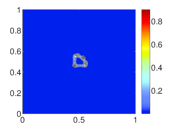
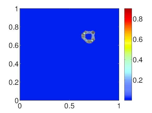
Absolute value of error
Simulation Results
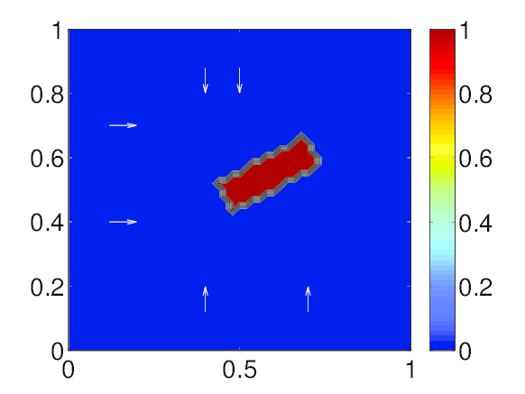
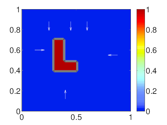
Actual map
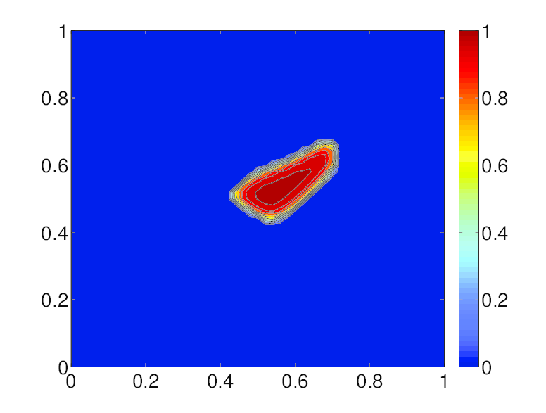
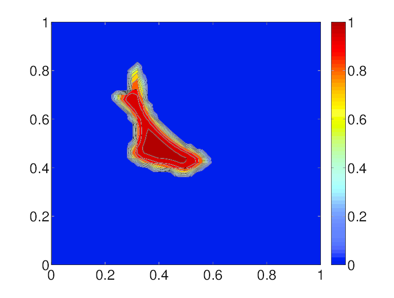
Estimated map
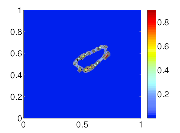
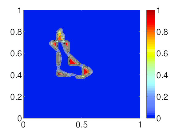
Absolute value of error
A Probabilistic Topological Approach to Quantifying Environmental Features*
*Ragesh K. Ramachandran, Sean Wilson, and Spring Berman. A probabilistic topological approach to feature identification using a stochastic robotic swarm. In To appear in the Int’l. Symposium on Distributed Autonomous Robotic Systems (DARS), 2016
Problem Statement
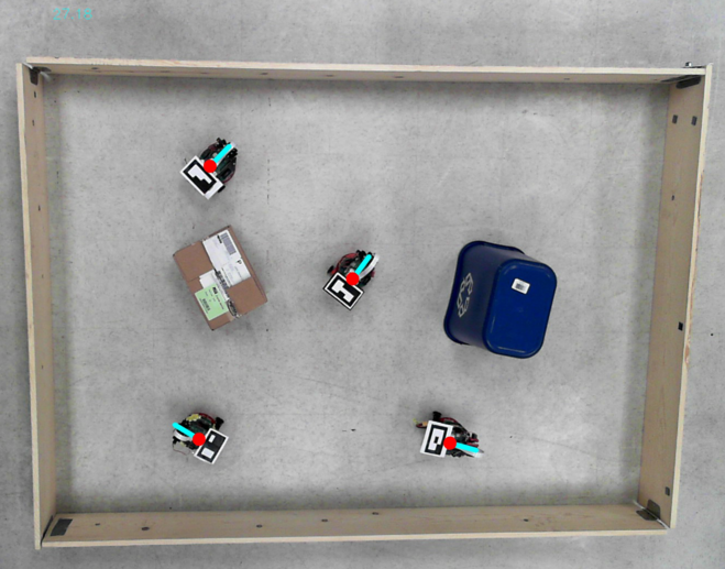
We consider the problem of mapping a bounded, unknown, GPS-denied 2D environment using a swarm of N robots.
The focus of the research is to find a scalable method to extract the map from the information obtained by resource constrained robots.
Related Work
Our previous work, Ramachandran et al.(2015) uses a PDE based model of the swarm to solve the problem. But requires large number of robots.
Ramaithitima et al.(2016) propose an algorithm that covers the free space of the environment with robots and then constructs an approximate generalized Voronoi graph. But requires communication.
In Dirafzoon et al.(2015) persistent homology is applied on a point cloud of the domain’s free region based on encounter time with robots. But each robot requires identification label.
Current focus
As a first step to solve this problem, we quantify the topological features (holes or obstacles) in the domain.
Types of Scenarios
Type I: Robots receive accurate estimates of their global positions when they are close to the boundary of the domain.
Type II: Robots do not receive global position updates anywhere in the domain.
Robot Motion Model
The displacement of a robot over a time step $\Delta t$ is given by: $$\mathbf{X}(t + \Delta t) = \mathbf{X}(t) + \mathbf{V}(t)\Delta t + \mathbf{W}(t)$$
Where,
$$\mathbf{V}(t) = [v_x(t),\ v_y(t)]^T = [v\ \cos(\theta(t)), \ v\ \sin(\theta(t))]^T$$ $$\mathbf{X}(t) = [x(t),\ y(t)]^T$$ $\mathbf{W}(t) \in \mathbb{R}^2$ is a zero mean Gaussian random vector
Robot Data
Data that robot $j \in \{1,...,N\}$ obtains at time $t_k \in [0, T]$, $k \in \{1,...,K\}$, consists of the element $d^j_k = \{\mu^j_k, \Sigma^j_k\}$.
$\mu^j_k \in \mathbb{R}^{2}$ is the mean of the robot's estimate of its $(x,y)$ position.
$\Sigma^j_k \in \mathbb{R}^{2\times2}$ is the covariance matrix of its position estimate.
Both at time $t_k$
Processing the Data
Discretize the domain into a high-resolution uniform grid. $m_i$ denotes a grid cell.
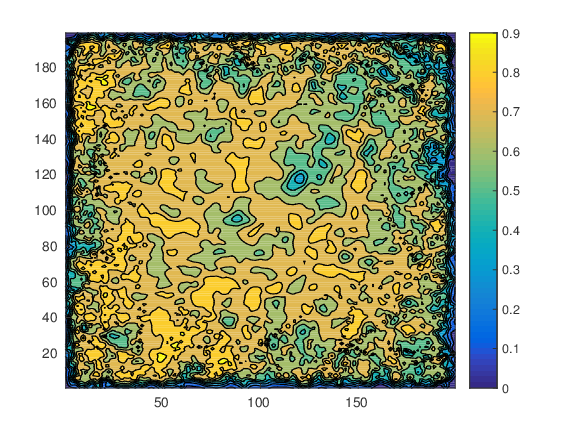
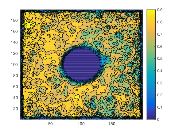
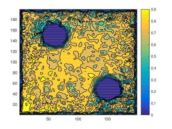
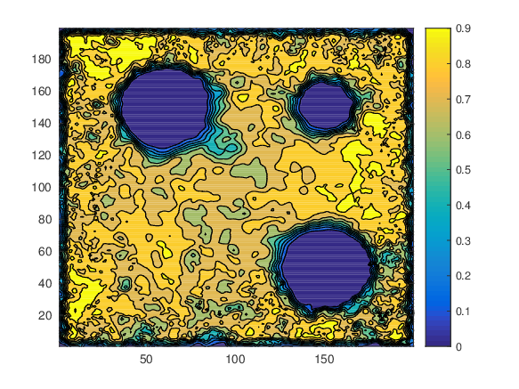
Use the robots' data to assign each grid cell $m_i$ a probability $p^f_i$ of being free.
Integrate the Gaussian distribution with mean $\mu^j_k$ and covariance matrix $\Sigma^j_k$ over the cell region to obtain $p^f_i$.
Processing the Data
Assign a score $s_i \in [0, \infty)$ to each grid cell $m_i$. $s_i = \frac{1}{\left | P_i \right |}\sum _{p \in P_i} \log\left ( \frac{1}{1 - p} \right )$. Where $P_i = \{p_{ijk} ~|~ p_{ijk} > \rho, \rho > 0\}$ and $p_{ijk}$ is computed using the $k^{th}$ data element of the $j^{th}$ robot.
Finally, $p^f_i$ of each grid cell being free is computed as $p_{i}^{f} ~=~ 1 - (\exp(s_i))^{-1}$.
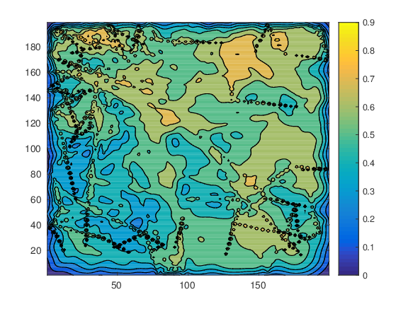
Probability map for TYPE I environment in Simulation
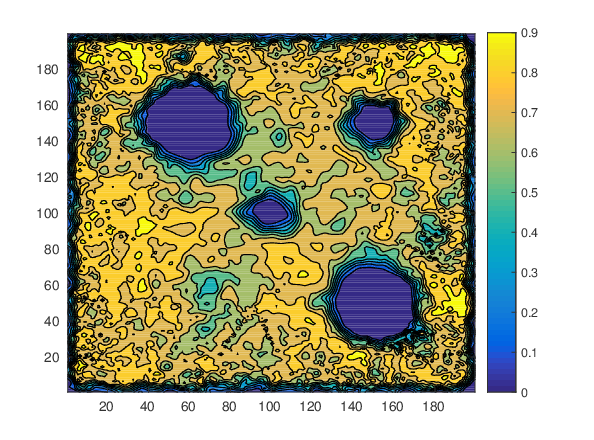
Actual Maps
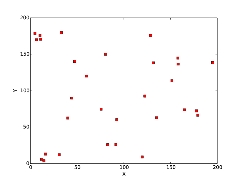
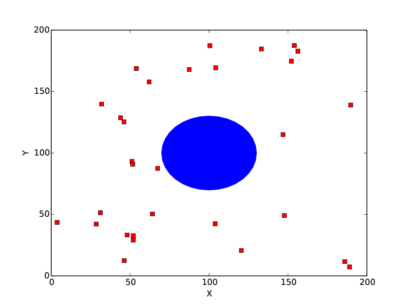
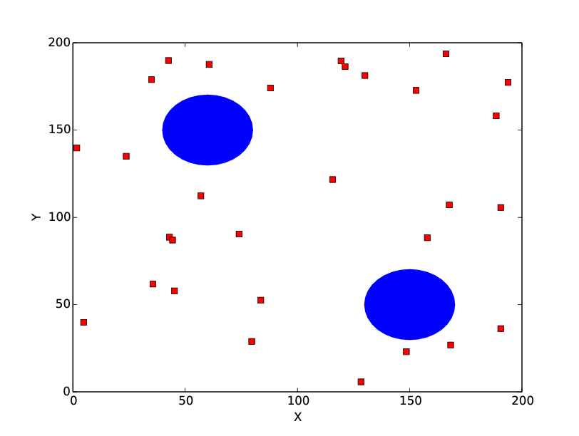
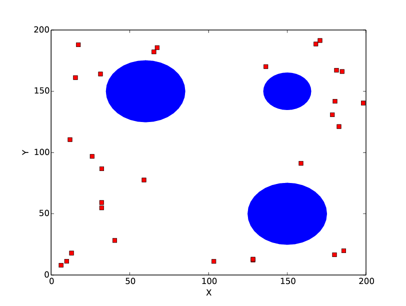
30 point robots deployed for 200 seconds
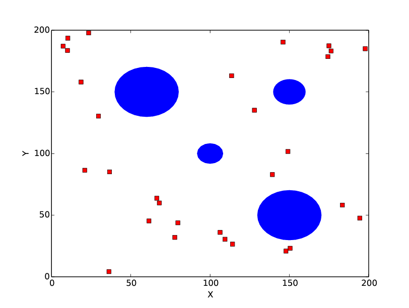
Probability map for TYPE II environment in Simulation
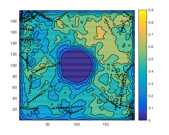
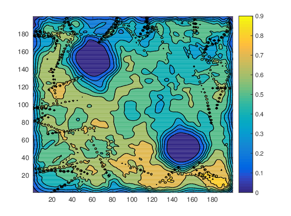
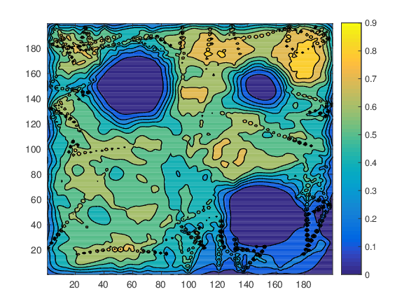
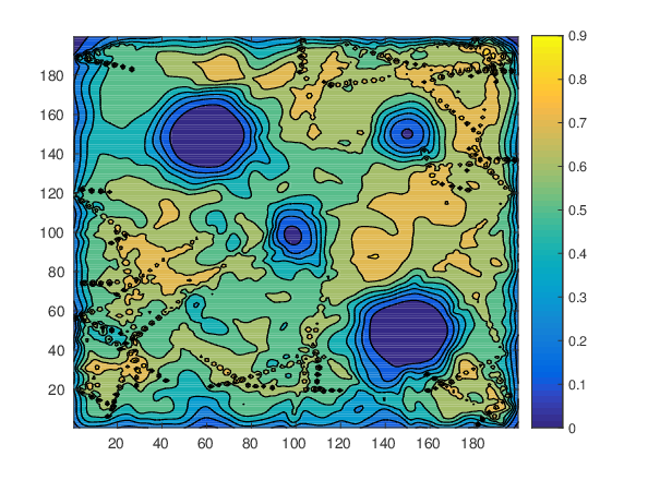
Actual Maps


30 point robots deployed for 200 seconds
Finding the Number of Features or Obstacles
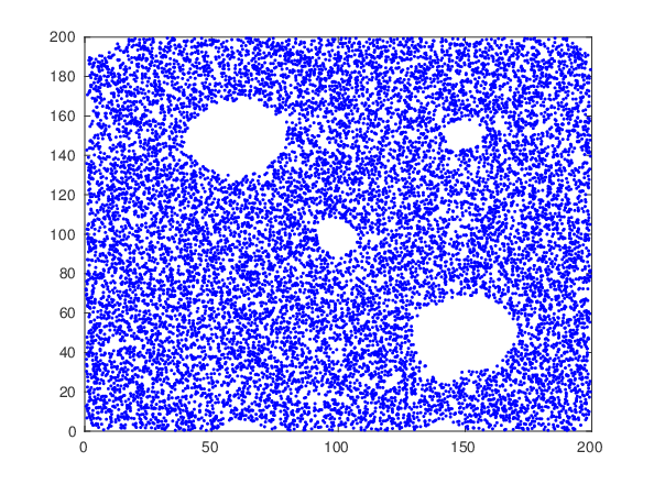
Point cloud is obtained by sampling a dense, uniformly random set of points from the domain based on a probability map of the domain and rejecting those points that are inside a grid cell whose $p^f_i$ is below a given threshold.
Landmark points are selected from the point cloud using the sequential max-min algorithm.
Finally, a Rips complex based filtration is constructed from landmark points and barcode diagrams are extracted.
The procedure was tested for Type I & Type II scenarios.
Rips complex based filtration
Background (Algebraic Topology)
vectors $v_0, v_1, ..., v_k \in \mathbb{R}^n$ are affinely independent if the vectors $ v_1 - v_0, ..., v_k - v_0 $ are linearly independent.
A $k$-simplex $\sigma \subset \mathbb{R}^n$ can be defined as the convex hull of $k+1$ affinely independent vectors $\{v_0, v_1, ..., v_k\}$, called vertices. $\sigma = [v_0, v_1, ..., v_k]$
A face $\tau$ is the convex hull of a subset of $\{v_0, v_1, ..., v_k\}$
A simplicial complex $\kappa$ is defined as a finite collection of simplices $\sigma$.
Illustration

Background continued...
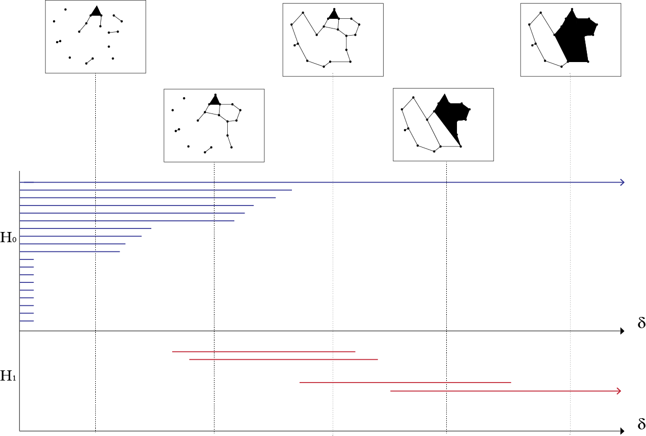
Rips complex is formed by choosing a parameter $\delta > 0$ and adding a $k$-simplex to the simplicial complex if every vertex in the simplex is within a distance $\delta$ from every other
If $f: \kappa \to \mathbb{R} $ is a function such that $\tau \leq \sigma$ implies that $f(\tau) \leq f(\sigma)$, then $f^{-1}((-\infty, \delta])$ is a simplicial complex denoted by $\kappa_\delta$ and $\delta_1 \leq \delta_2$ implies that $\kappa_{\delta_1} \subseteq \kappa_{\delta_2}$, yielding a filtration of simplicial complexes with $\delta$ as the filtration parameter.
A barcode diagram is a graphical representation used to identify the persistent topological features
Rips complex based filtration with barcode
Point Cloud and Landmark Points for TYPE II environment
Point cloud
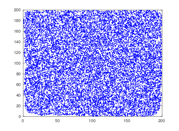
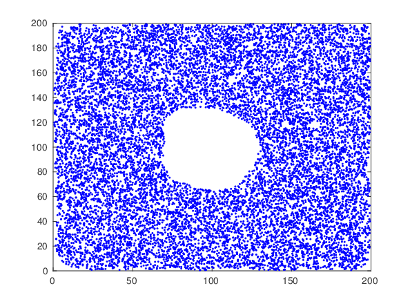
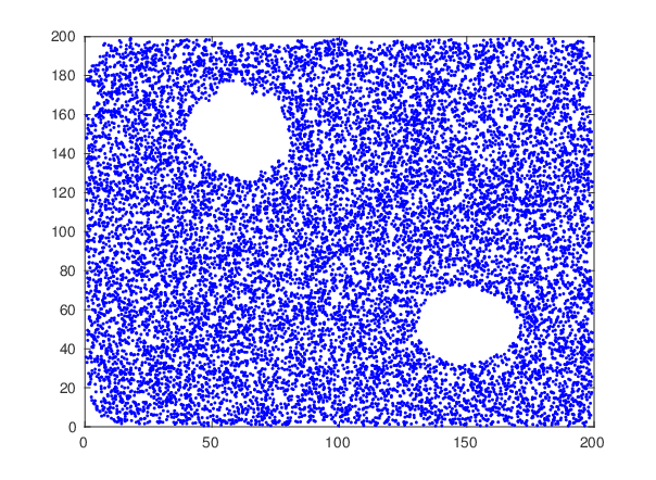
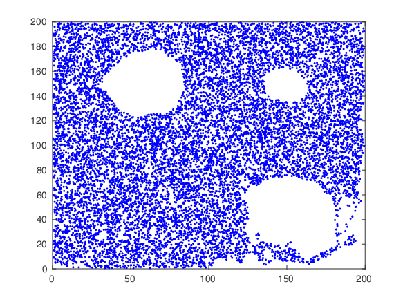
Landmark Points
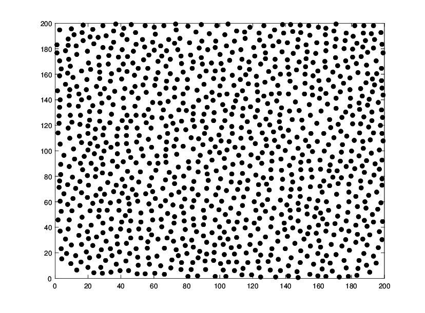
No features
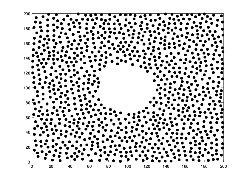
One feature
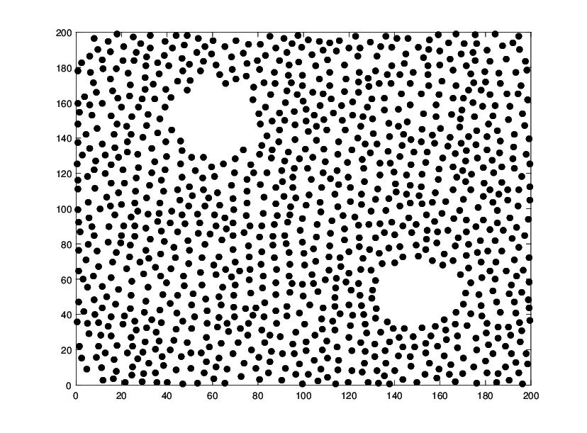
Two features
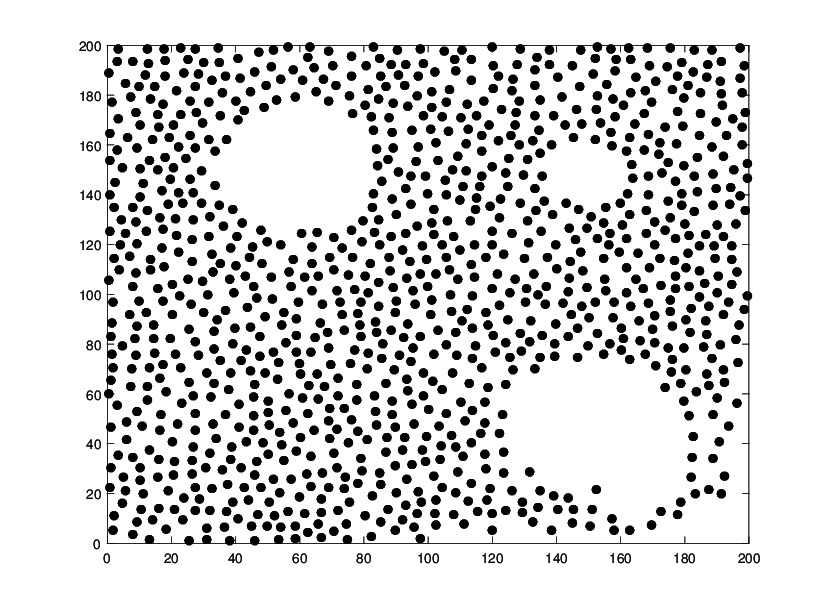
Three features
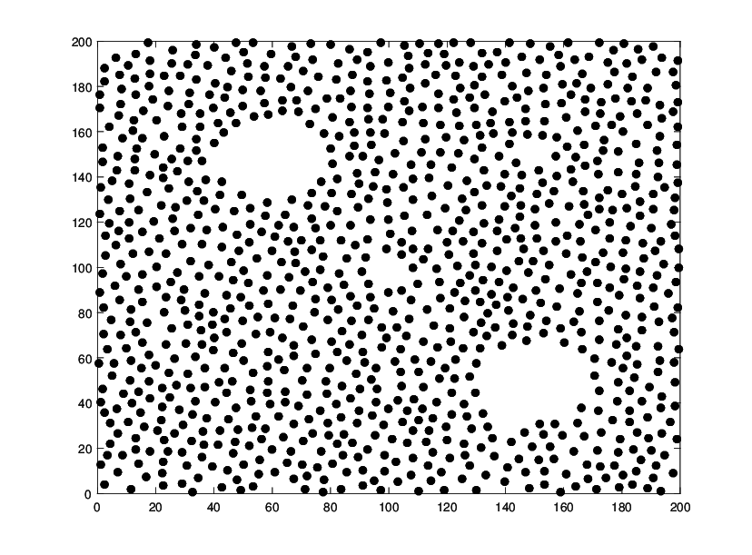
Four features
Point Cloud and Landmark Points for TYPE I environment
Point cloud
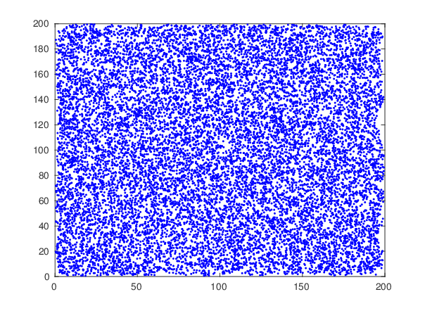
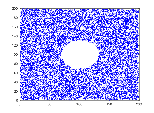
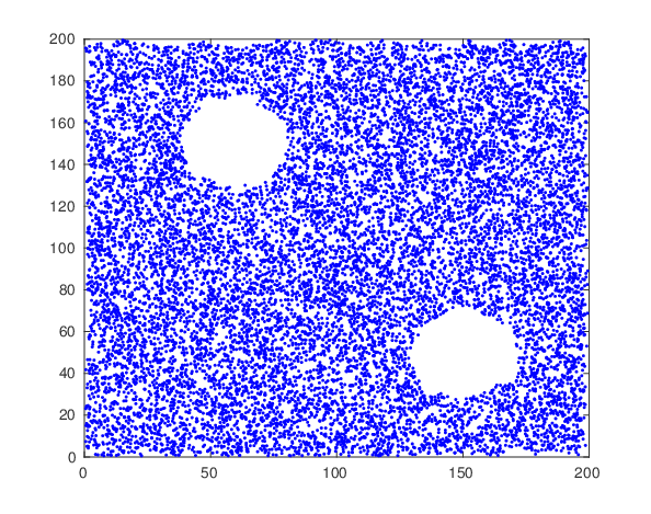
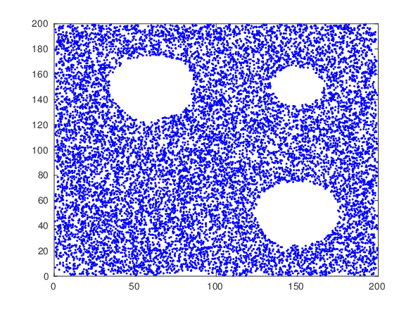
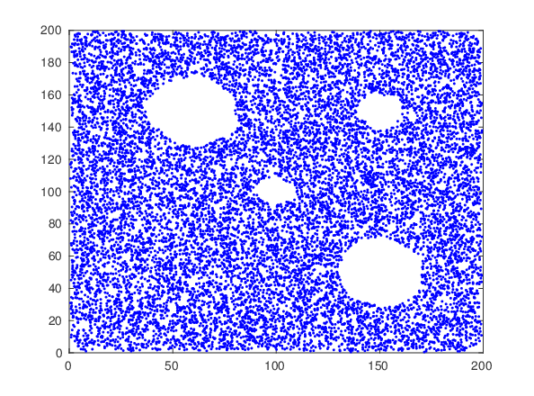
Landmark Points
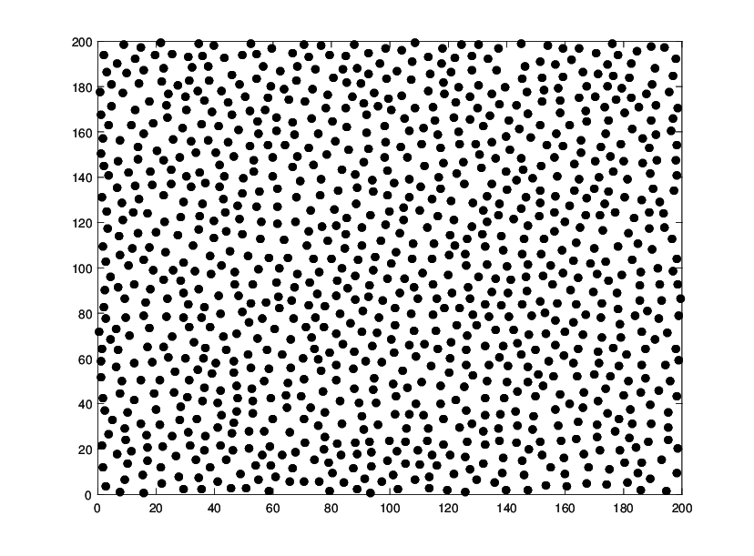
No features
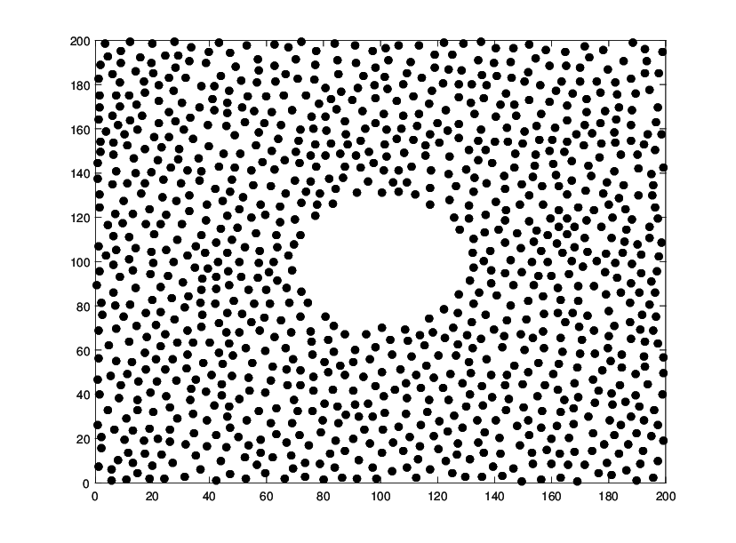
One feature
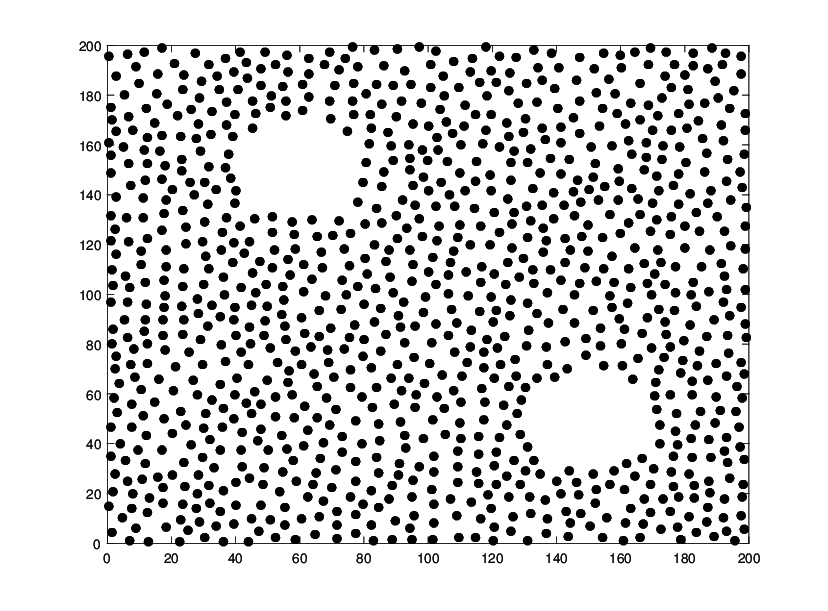
Two features
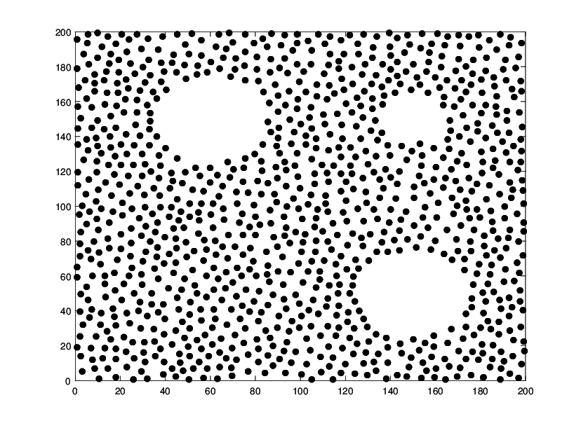
Three features
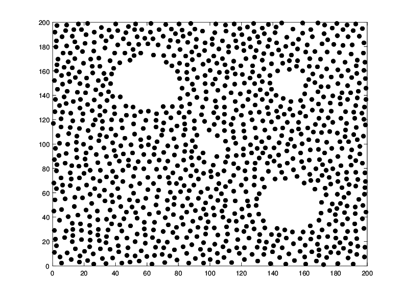
Four features
Barcode Diagram TYPE II environments

No features

One feature
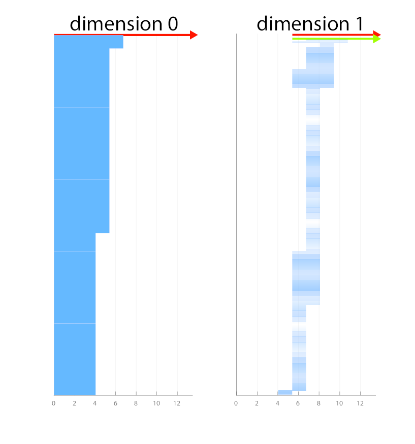
Two features
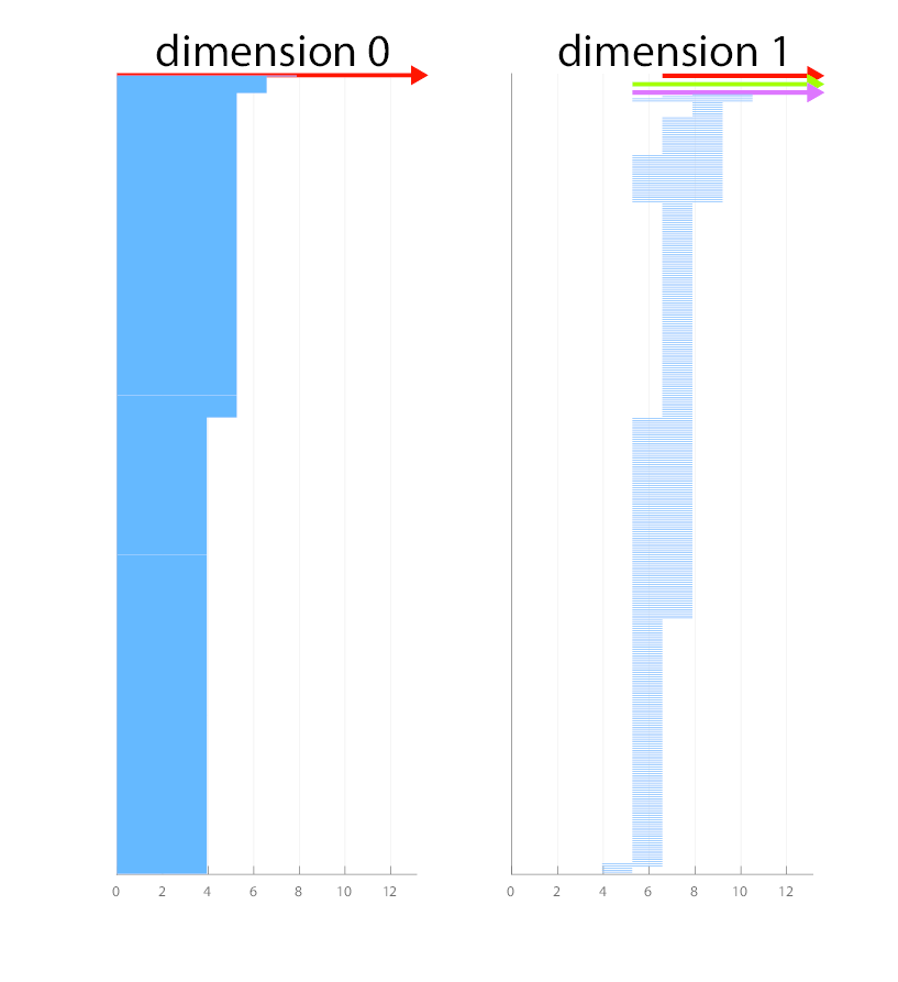
Three features

Four features
Barcode Diagram TYPE I environments
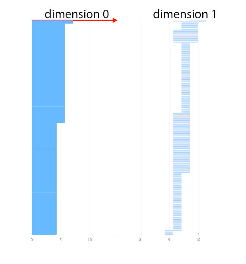
No features
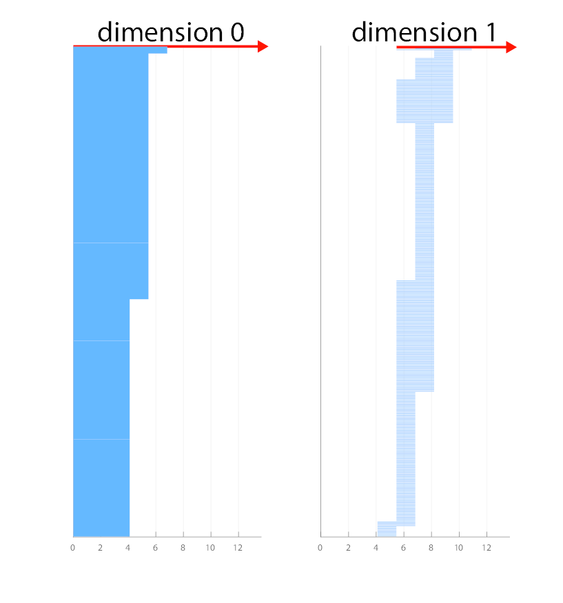
One feature
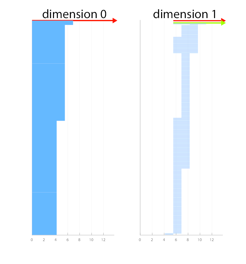
Two features
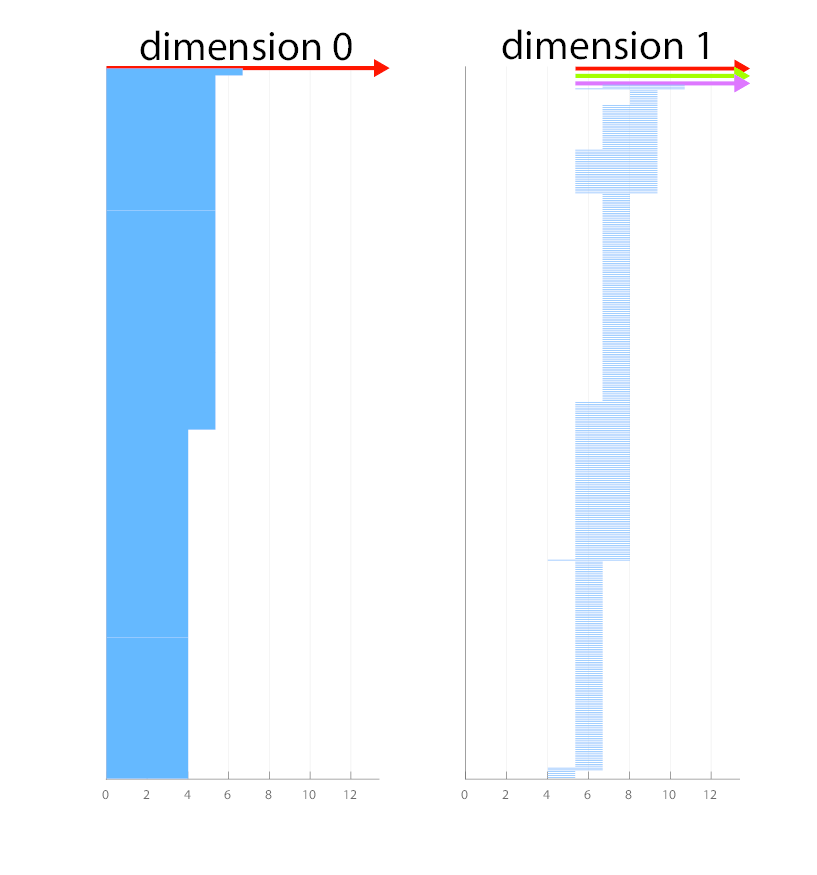
Three features
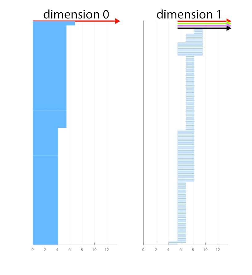
Four features
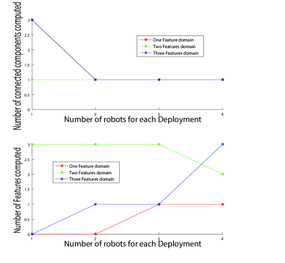
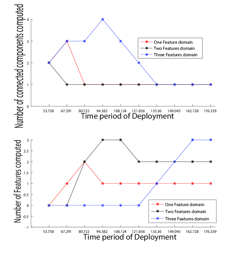
Effect of varying time of deployment on estimation
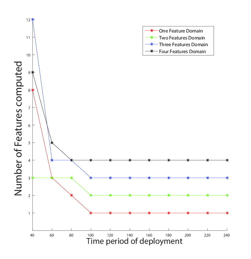
30 point robots deployed for each simulation
Effect of varying number of robots on estimation
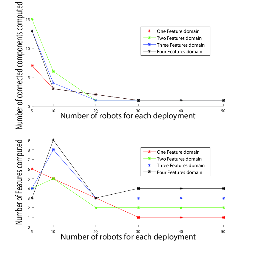
Time of deployment for each simulation : 200 seconds
Experiments on TYPE II environment
Experimental Setups
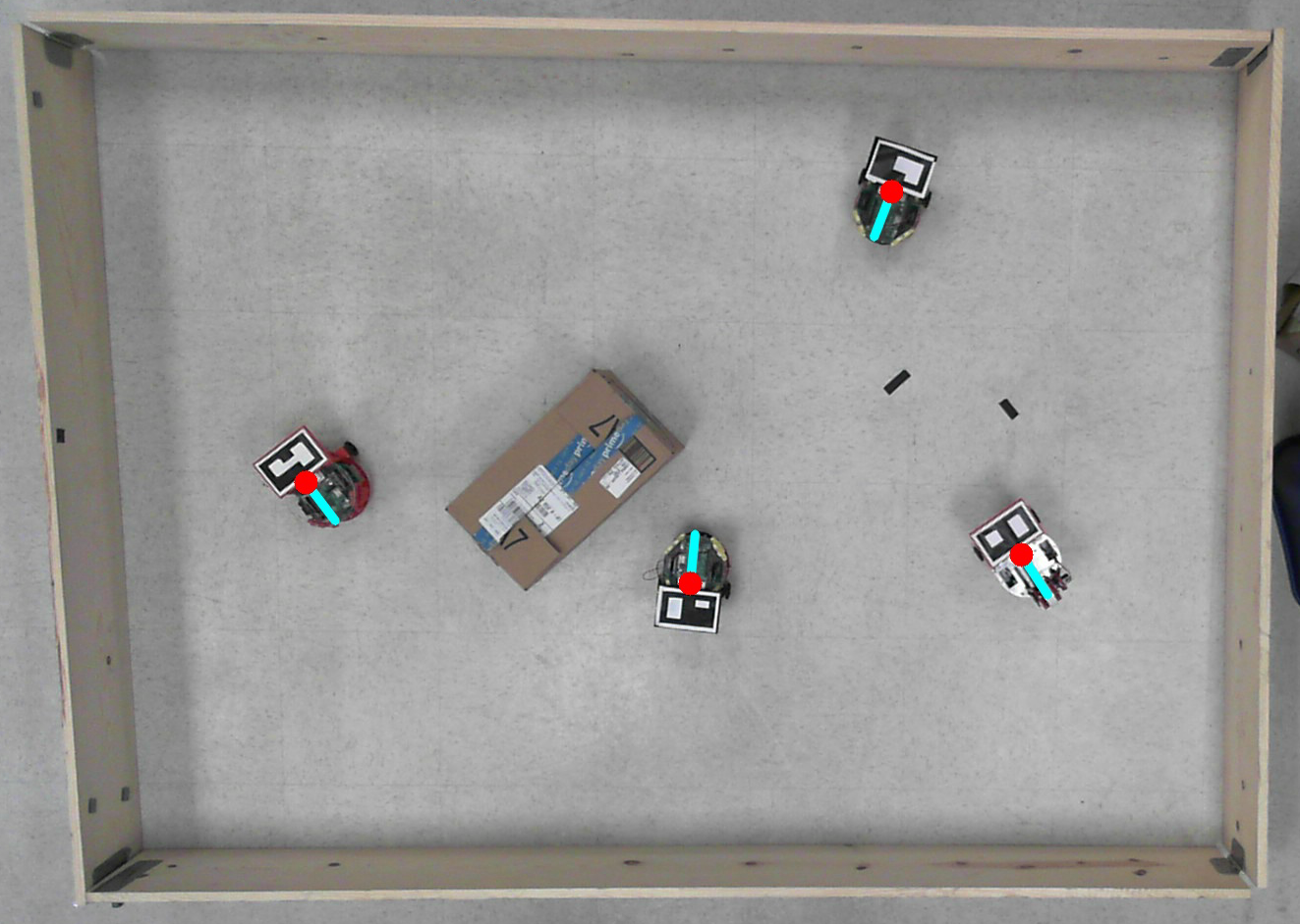
One feature
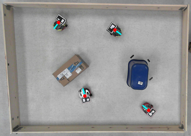
Two features
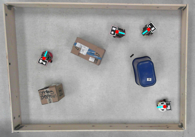
Three features
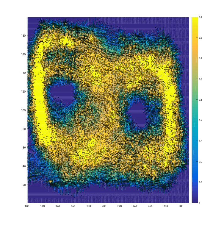
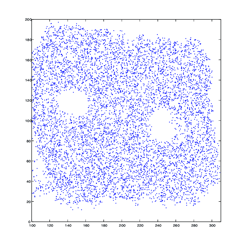
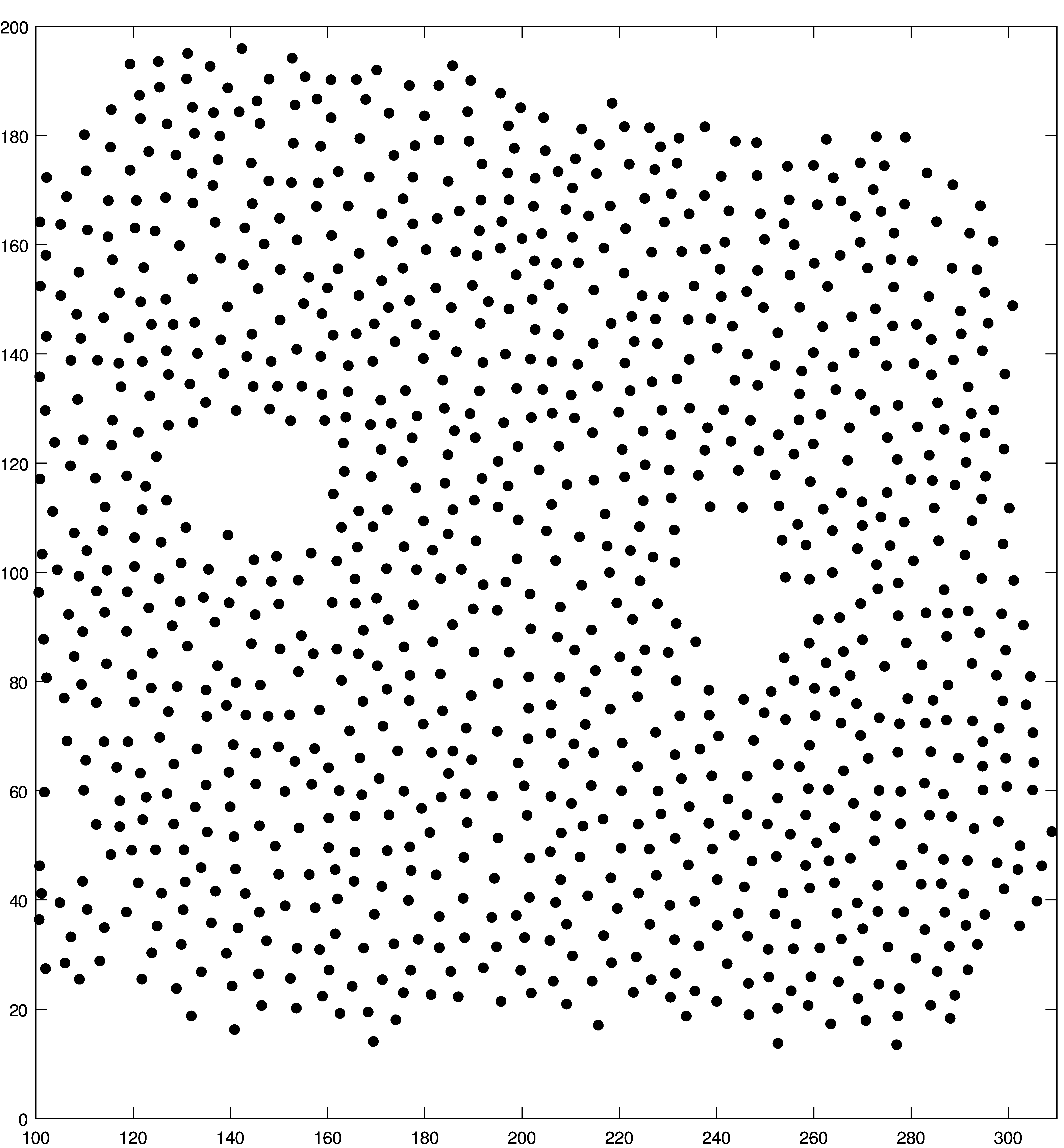
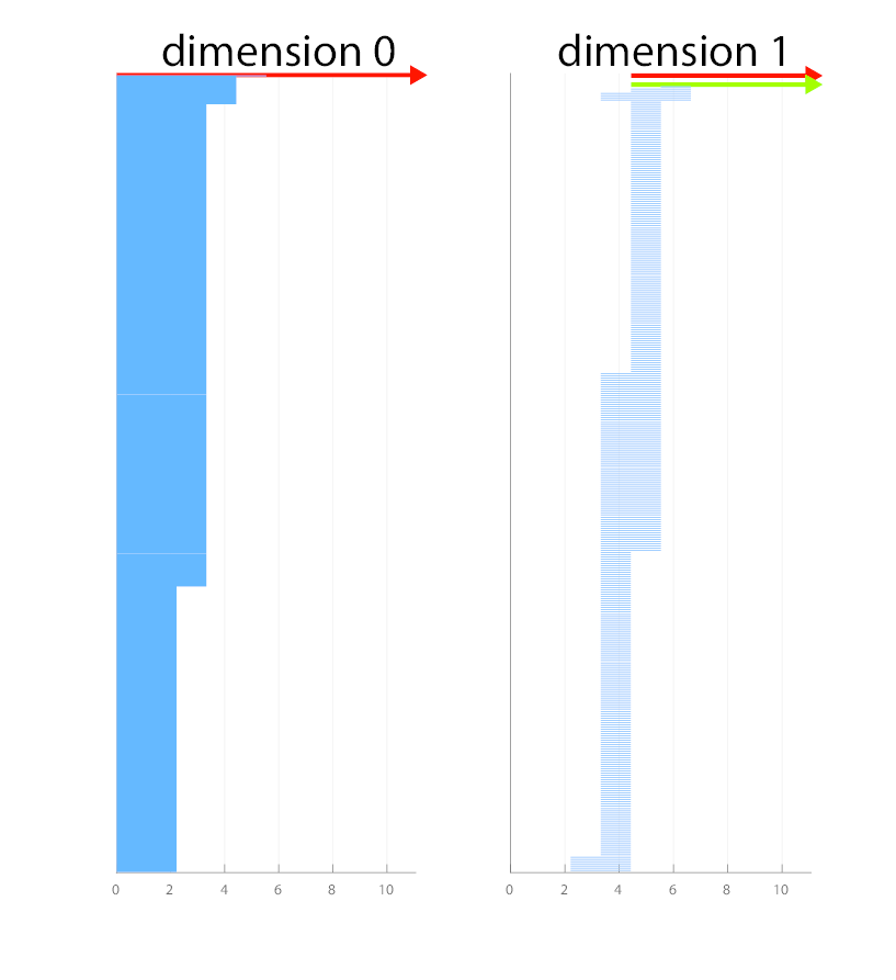
An Experimental Illustration

 Barcode
*4 robots deployed for 180 seconds
Experimental Validation of Estimation
A Probabilistic Approach to Constructing Topological Maps of an Environment*
*Ragesh K. Ramachandran, Sean. Wilson, and Spring. Berman. A probabilistic approach to automated construction of topological maps using a stochastic robotic swarm. IEEE Robotics and Automation Letters, 2(2):616–623, April 2017.
Extension of the Previous work
What more can be done?
How to find an automated procedure to threshold the density function in order to isolate the obstacle region?
Can we build a topological map of the domain?
Topological Map Illustration
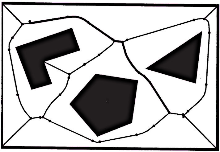
Topological map of a domain with three obstacles1
1Taken from Dr.Markus Haid blog
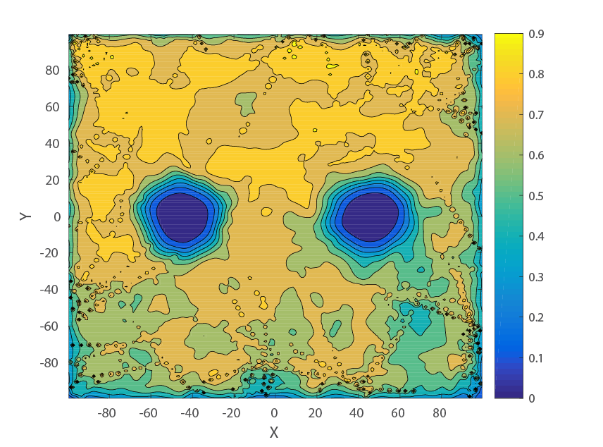
Compute Threshold And Identify Number Of Obstacles
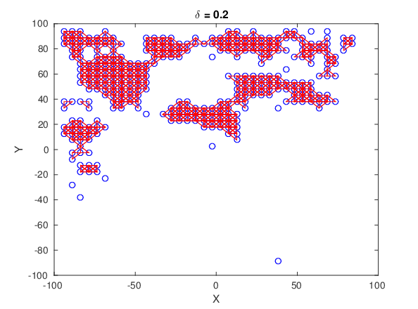
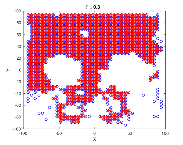
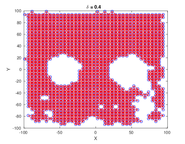
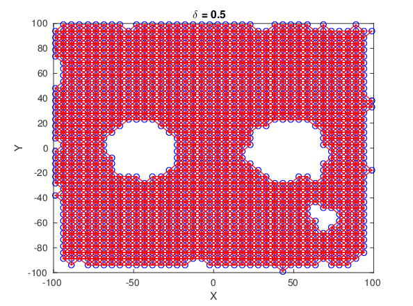
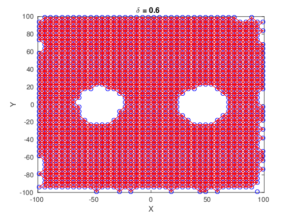
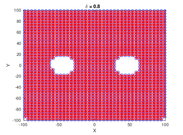
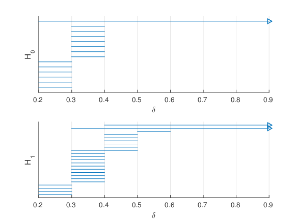
A filtration is generated by the thresholding the probability map and constructing a simplicial complex at each level and choosing $\delta$ = 1 − threshold ($\alpha$) as the filtration parameter
The barcode generated out of this filtration can be used to compute optimal threshold and identify number of obstacle.
Density Function Thresholding Based on Filtration
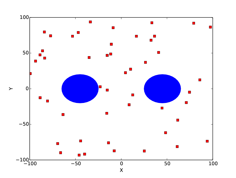
Actual Domain
Computed density function
Density Function Thresholding Based on Filtration
Simplicial complex for each filtration value
$\delta$ = 0.2
$\delta$ = 0.3
Density Function Thresholding Based on Filtration
Simplicial complex for each filtration value
$\delta$ = 0.4
$\delta$ = 0.5
Density Function Thresholding Based on Filtration
Simplicial complex for each filtration value
$\delta$ = 0.6
$\delta$ = 0.8
The Barcode From The Filtration
Obstacle Segmentation
The grid cells with $p^f_i < \alpha_{opt}$ belong to an obstacle.
Classify the grid cells in each obstacle and identify its boundary.
A graph is constructed with obstacle grid cell centers as vertices and the cells are classified by performing a BFS on this graph
The boundaries of each obstacle are identified as the elements in graph that belong to the same obstacle and have fewer than four neighbors.
Obstacle Segmentation Illustration
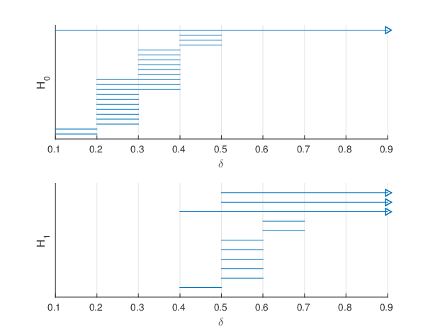
Barcode
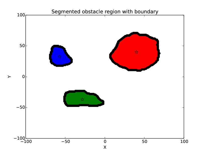
Segmented Obstacles and their Boundaries. The boundary is shown in black.
Topological Map Generation
A wave propagation algorithm is used to generate the approximate Generalized Voronoi Diagram(AGVD).
A graph is constructed in the same manner as the obstacle graph.
The algorithm is a modified form of Dijkstra's algorithm.
The algorithm outputs the set of vertices which constitutes the topological map of the domain in the form of a discrete AGVD.
Topological Map Video
Topological Map Results
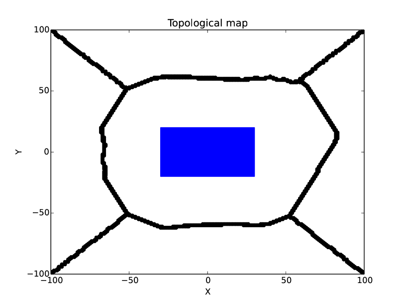
One Obstacle
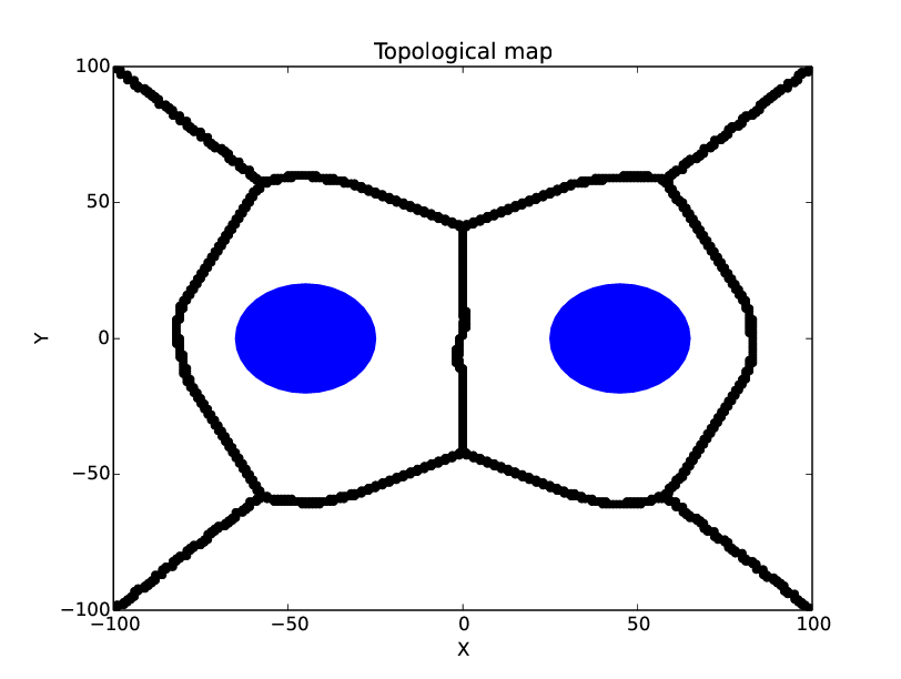
Two Obstacles
Topological Map Results
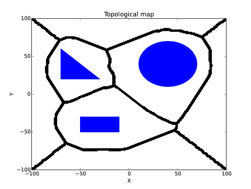
Three Obstacles
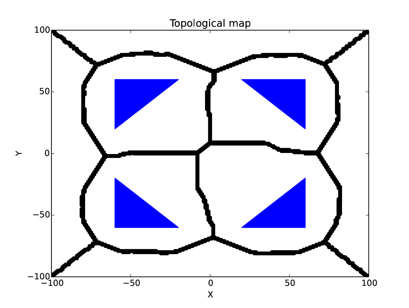
Four Obstacles
Experimental Illustration
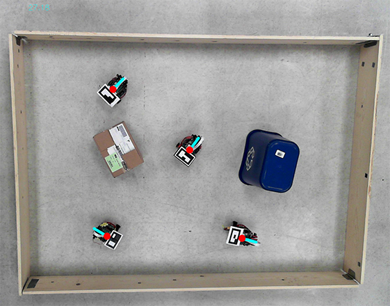
Experimental Setup with Pheeno robot platform1
1Sean Wilson et al., IEEE R-AL, July 2016
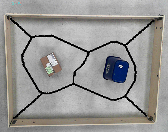
Map Overlaid on the Arena
Computational Complexity
Probability map generation: $\mathcal{O}(NKM)$, where $N$ robots each collect $K$ items of data over a domain that is discretized into $M$ grid cells.
Simplicial complex construction and barcode generation : $\mathcal{O}(M^{2.372})$, but for most practical applications it is close to $\mathcal{O}(M)$.
Obstacle segmentation : $\mathcal{O}(M)$.
AGVD extraction using the wave propagation algorithm :$\mathcal{O}(M\log{M})$.
Worst case complexity of the approach : $\mathcal{O}(M^{2.372})$.
Metric Map Construction using a Stochastic Robotic Swarm Leveraging Received Signal Strength*
*Ragesh K. Ramachandran and Spring Berman. Automated Construction of Metric Maps using a Stochastic Robotic Swarm Leveraging Received Signal Strength. In revision for IEEE Transactions on Robotics, 2018.
Problem Statement
We consider the problem of generating a metric map of a bounded, unknown, GPS-denied 2D environment using data collected by a swarm of N robots.
Extension of the Previous work
A robots are equipped with receivers to receive broad casted signals(wifi, bluetooth).
A mapping procedure is similar to the previous one, which is computing $p^f_i$ for each grid cell.
We prove the completeness of the mapping approach.
Updated Measurement Model
$$\mathbf{Z}(t) = \begin{bmatrix} \mathbf{S}(\mathbf{X}(t))\\ \mathbf{V}(t) \end{bmatrix} + \begin{bmatrix} \mathbf{N}_S(t)\\ \mathbf{N}_V(t) \end{bmatrix}$$$\mathbf{S}(\mathbf{X}(t)) = [S_1(\mathbf{X}(t)), ~...,~ S_l(\mathbf{X}(t))]^T$, $l$ number of transmitters(here $l = 2$).
$S_i(\mathbf{X}(t)) = K_i Pow_i ||\mathbf{X}(t) - \mathbf{X}_i||^{-\alpha}$, where $\alpha \in [0.1, 2]$, $Pow_i$ is the transmitted signal voltage of transmitter $i$
$\mathbf{N}_S(t) \in \mathbb{R}^l$ and $\mathbf{N}_V(t) \in \mathbb{R}^2$ as vectors of independent, zero-mean normal random variables.
Extended Kalman filter used.
Completeness of the Approach
Lemma: The error in the robots' position estimates is uniformly bounded, with a common bound for all robots, if each robot follows the previously mentioned motion model and estimates its state vector using an extended Kalman filter based on the outputs in $\mathbf{Z}(t)$.
Finally, we prove the existence of a threshold value of $p_{i}^{f}$ that distinguishes the free grid cells from the occupied cells.
Theorem: Under the assumption of complete coverage of the domain, a grid cell $m_i$ is free if and only if there exists a threshold $\gamma \in [0, 1]$ for which $p_{i}^{f} > \gamma$.
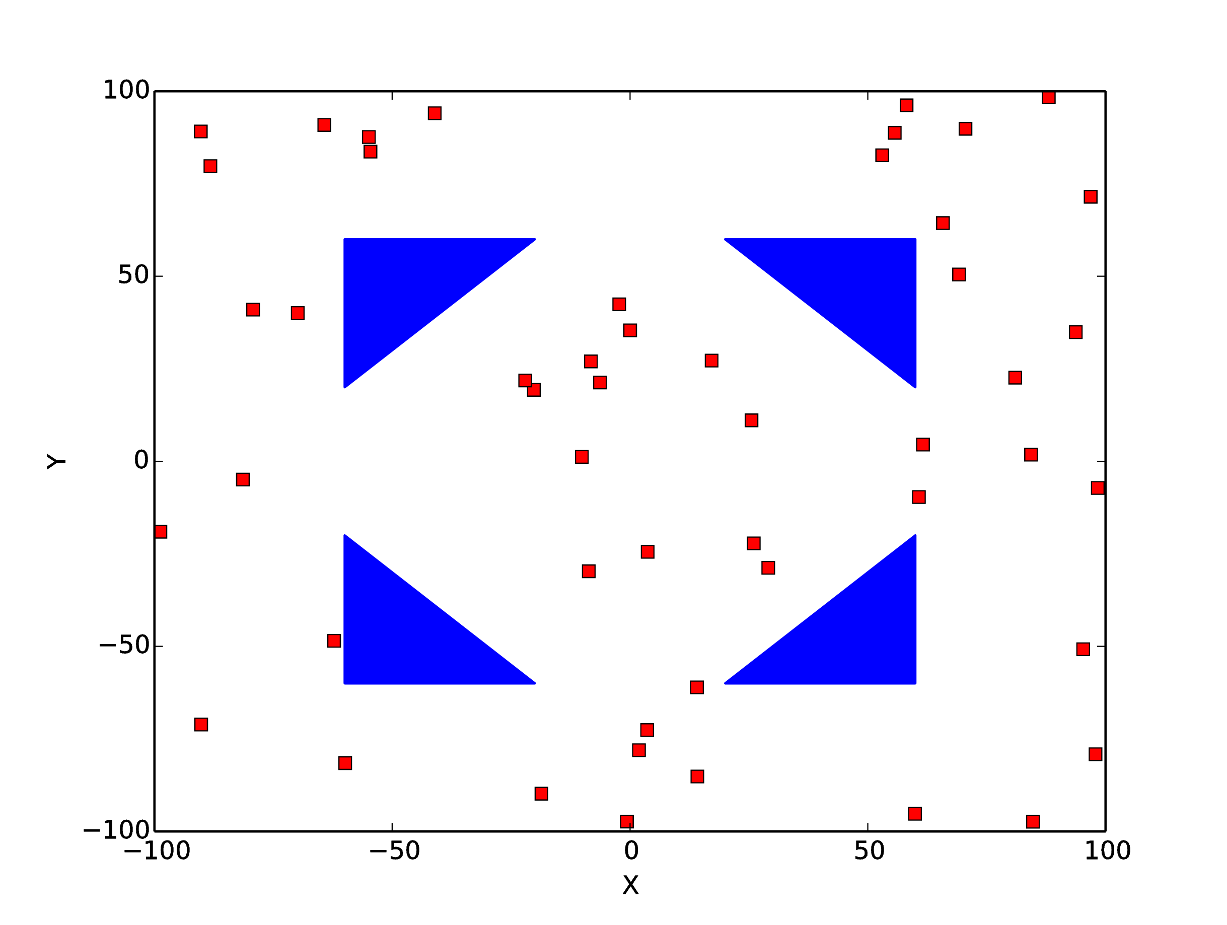
Actual Domain
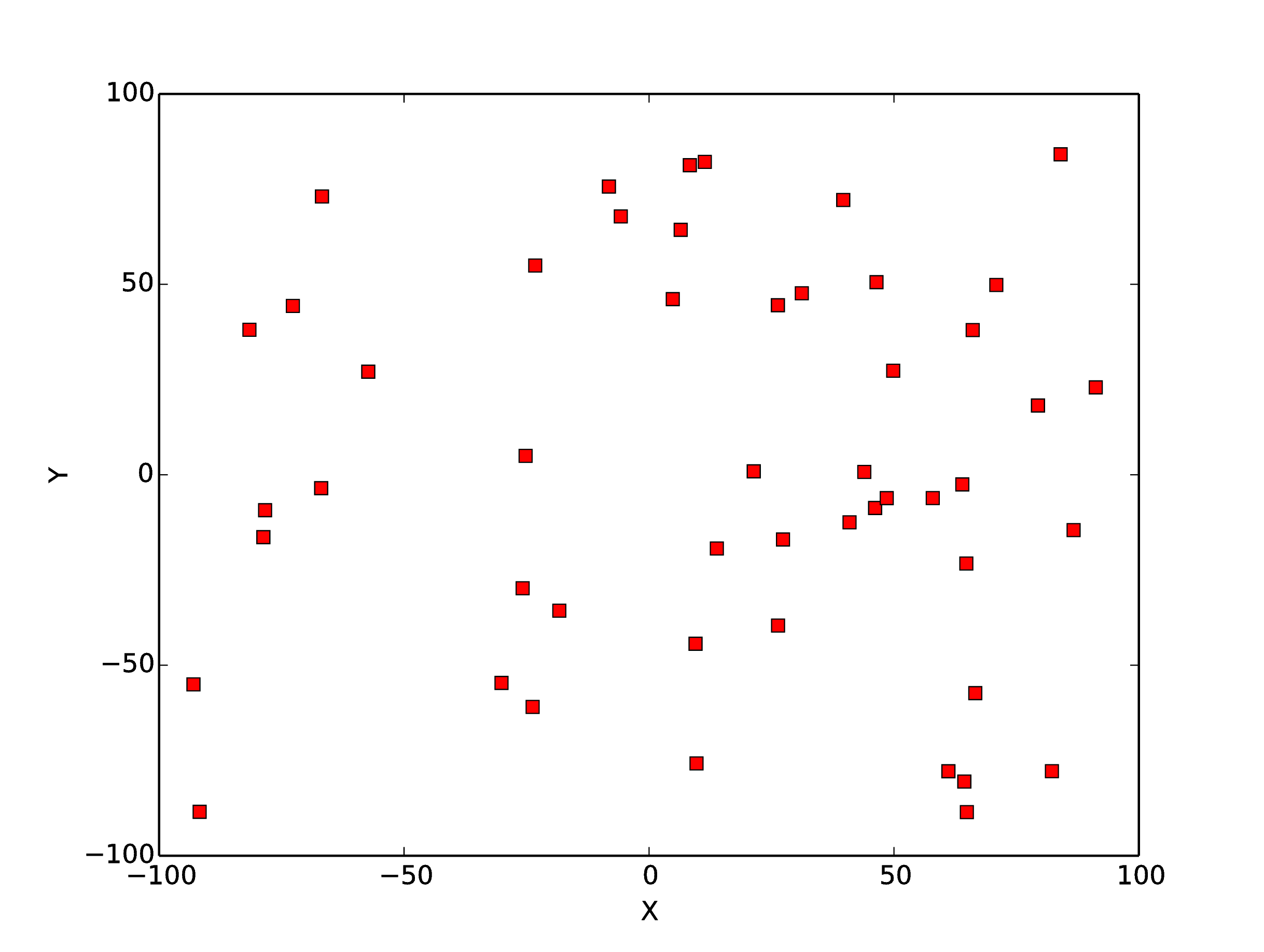
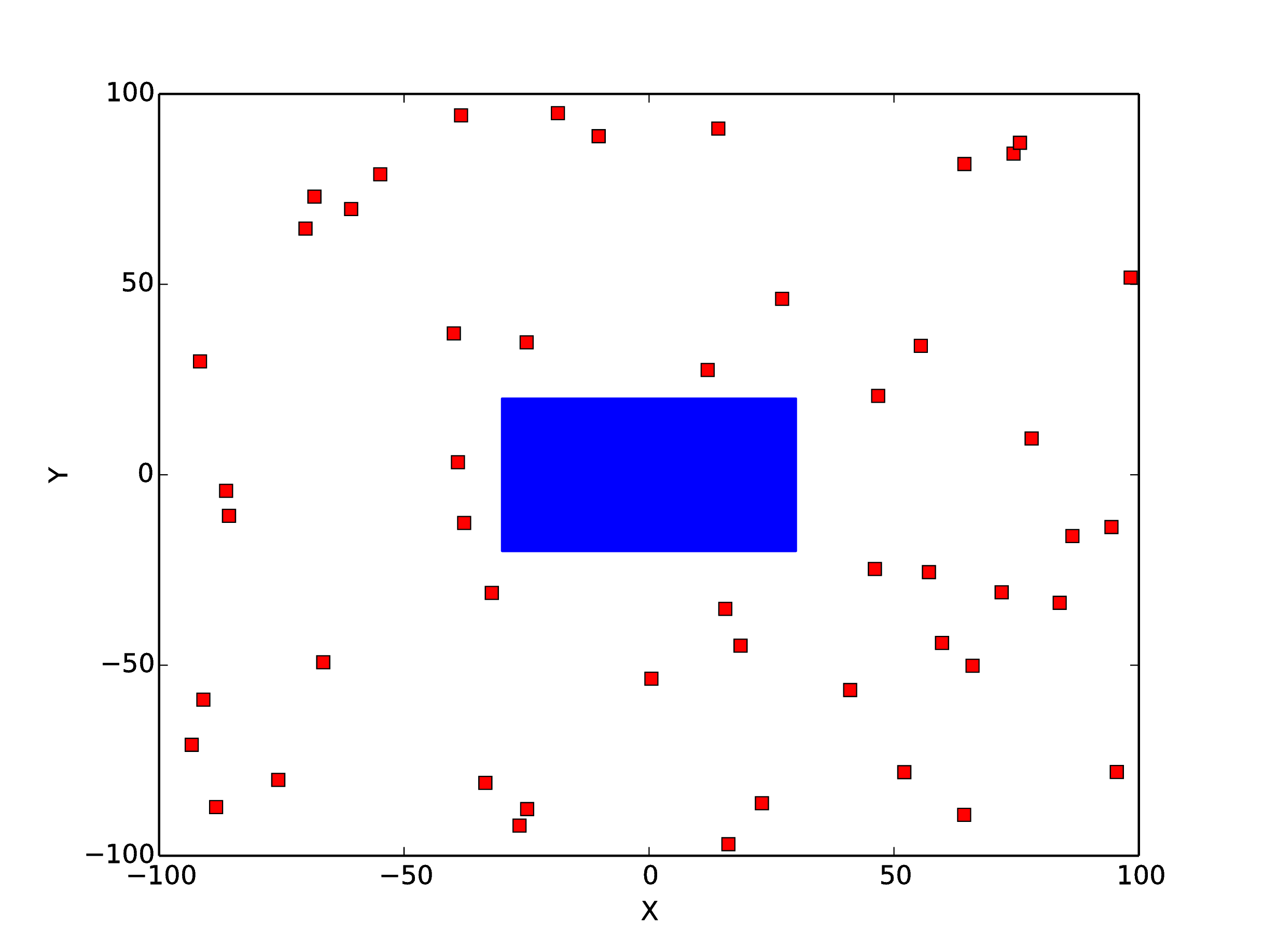
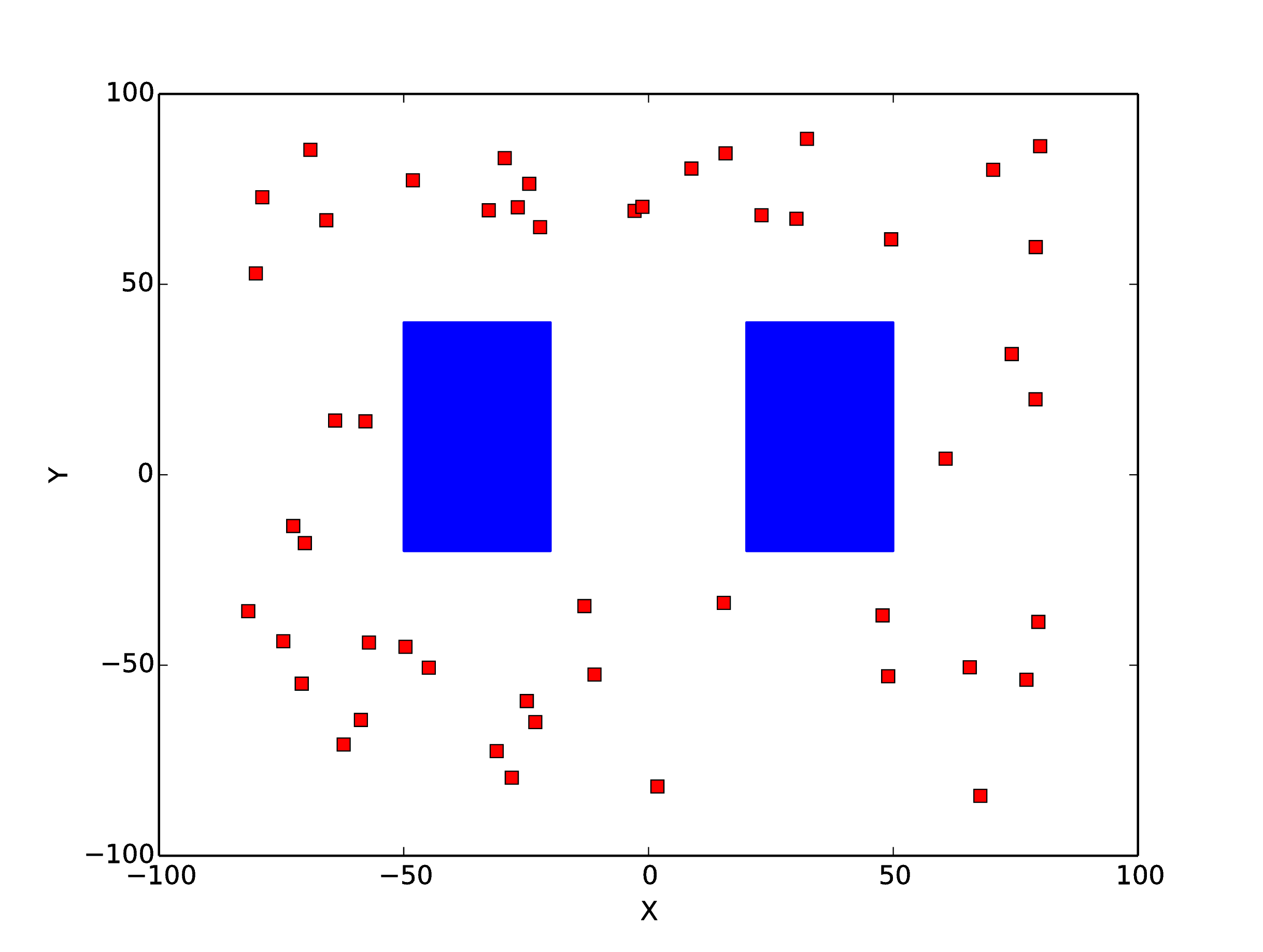
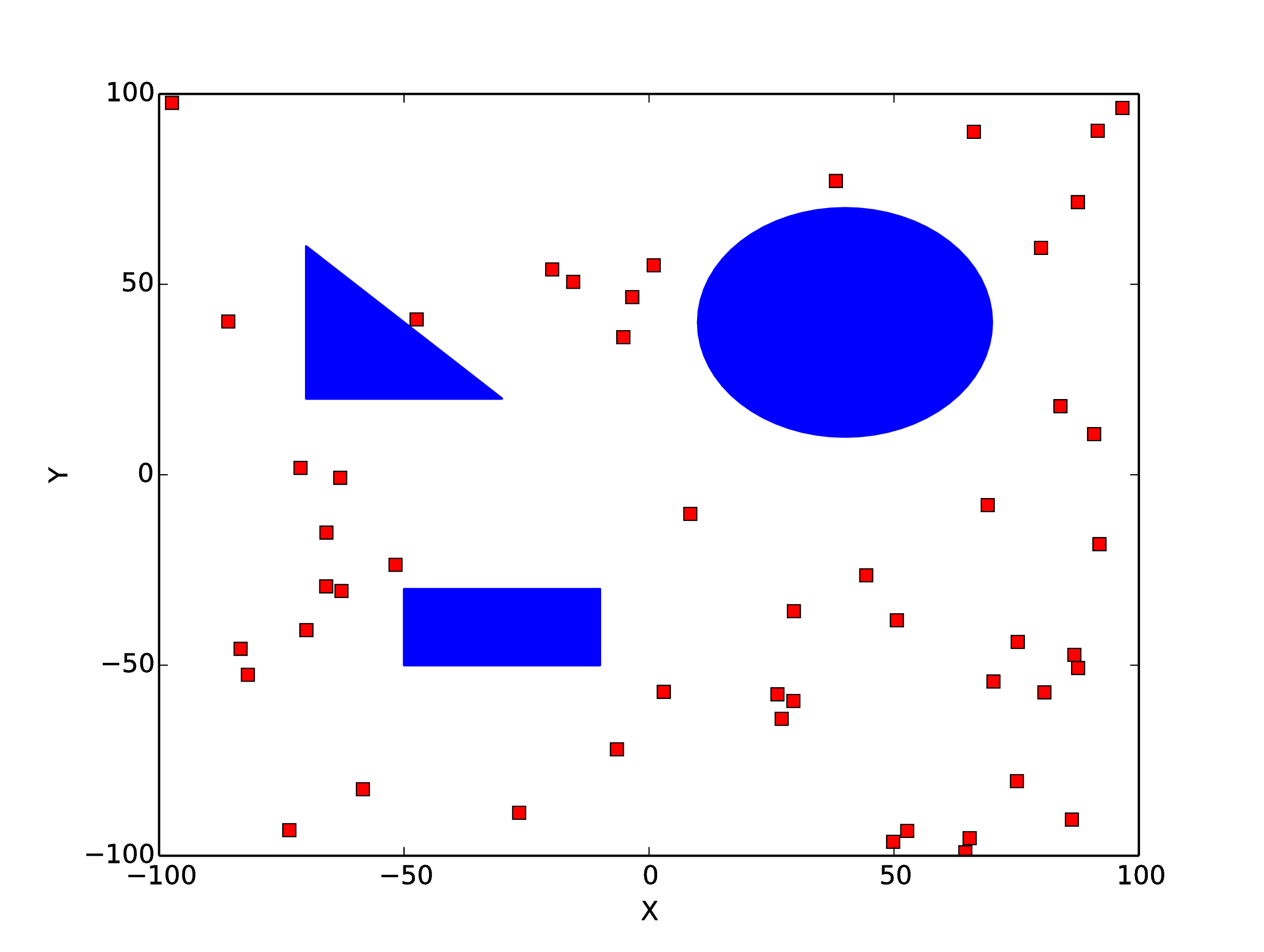
Probability map
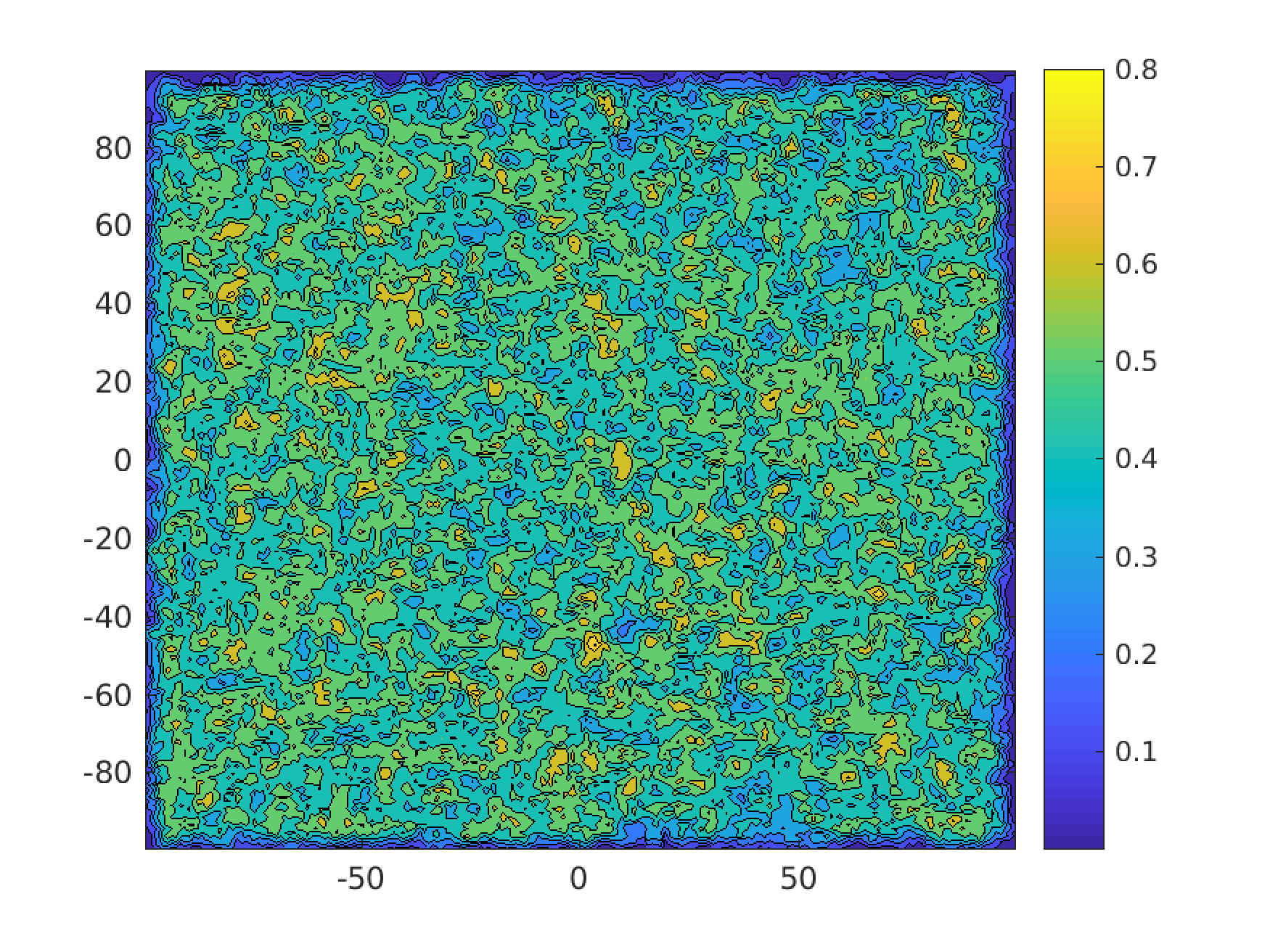
No features
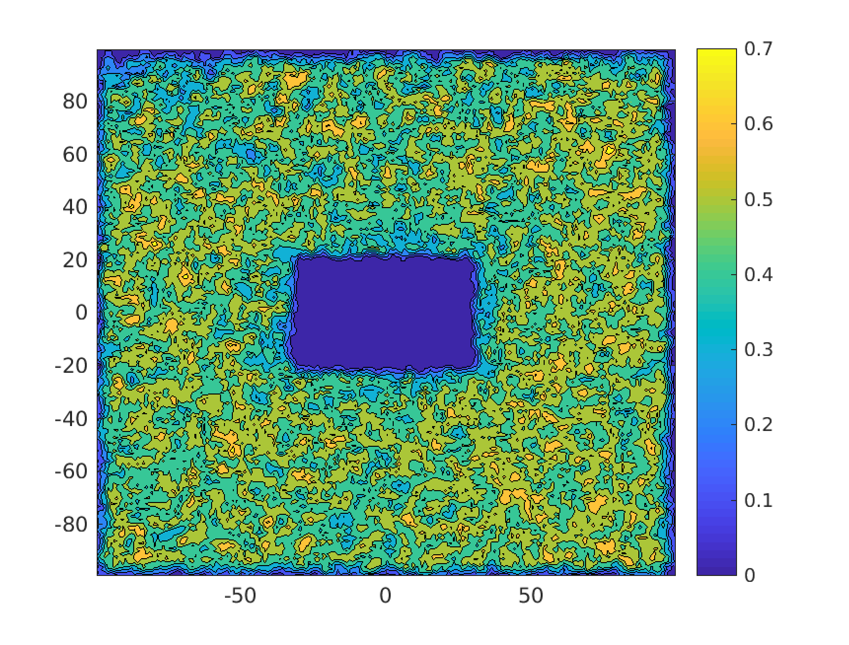
One feature
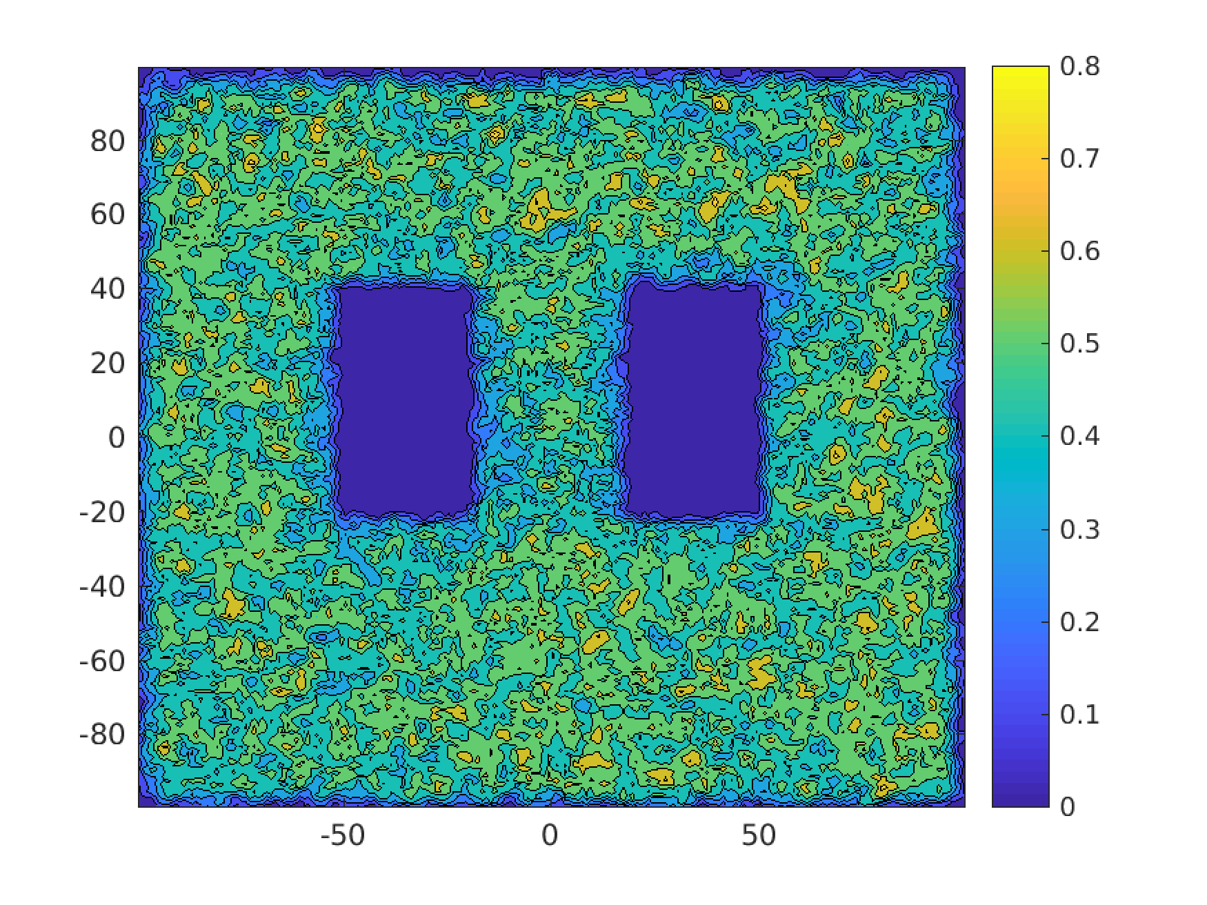
Two features
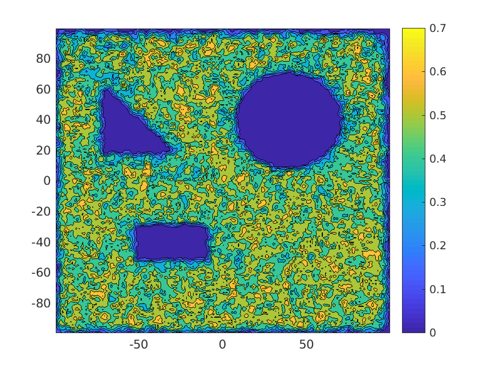
Three features
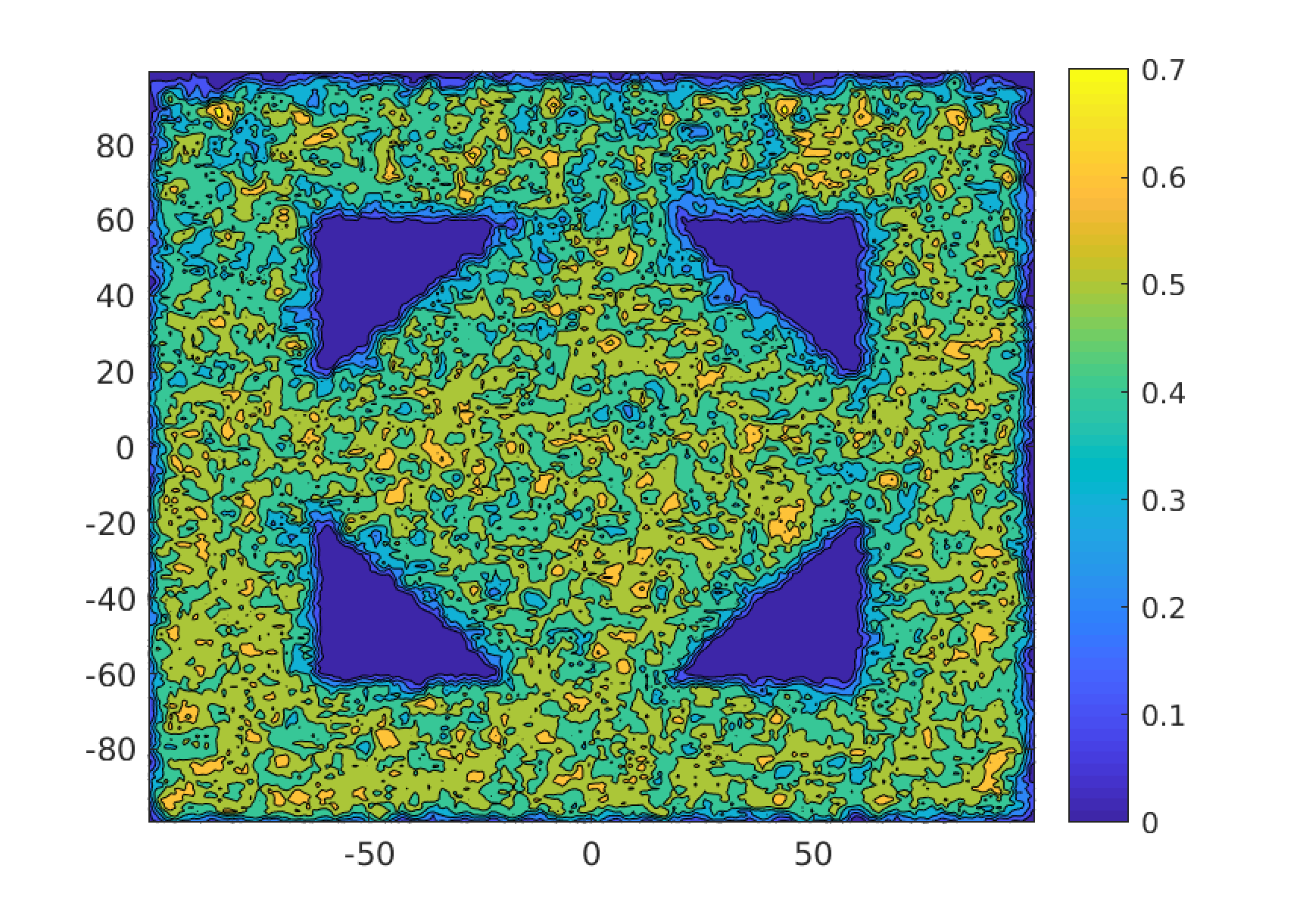
Four features
Thresholded map

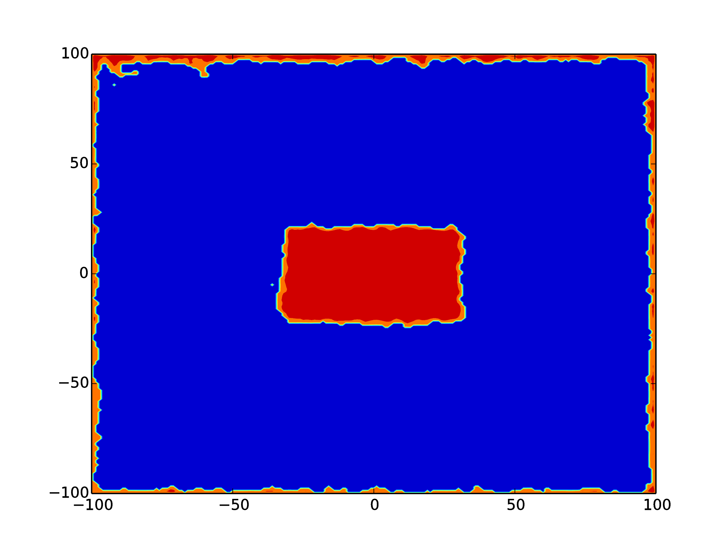
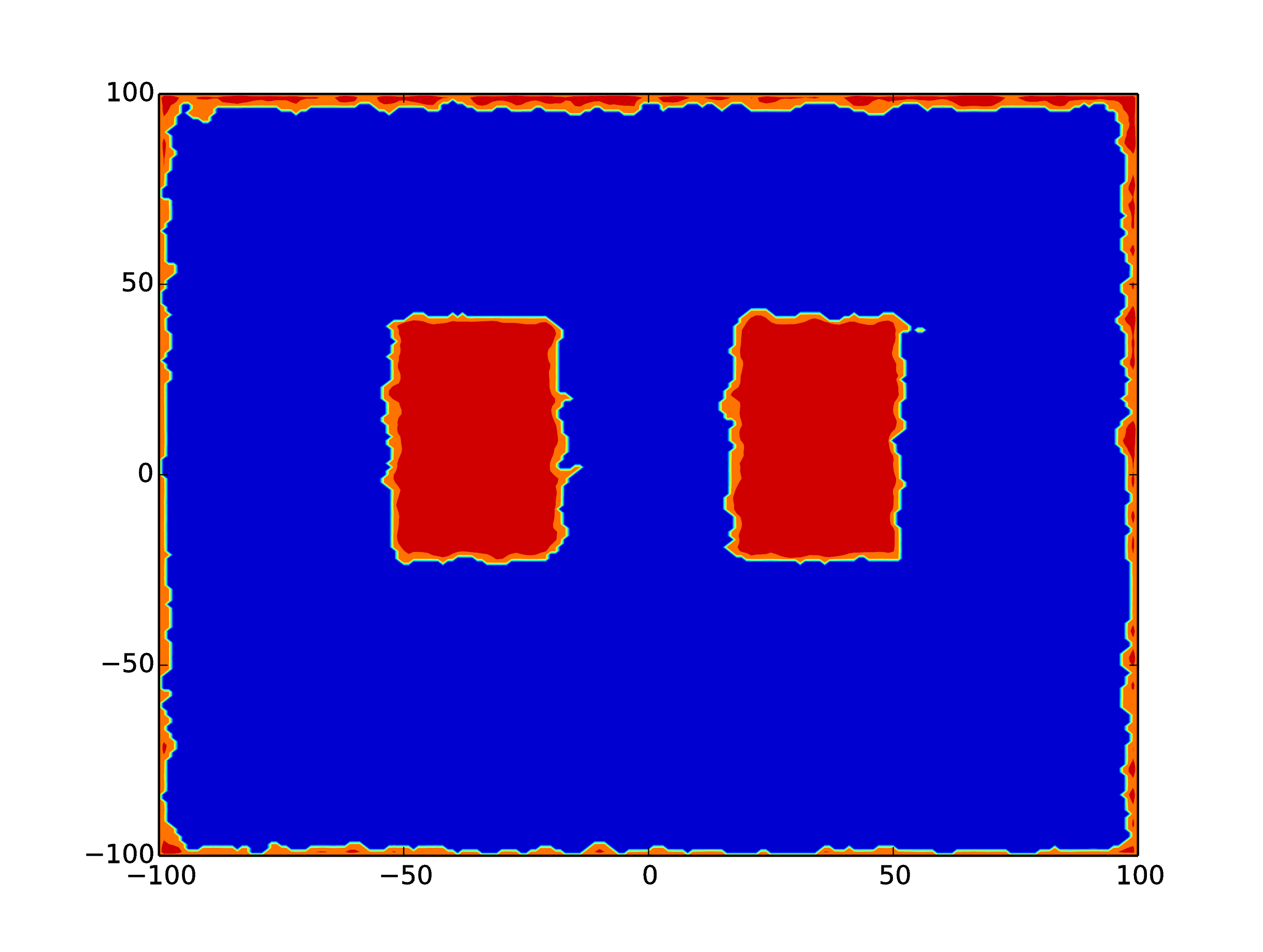
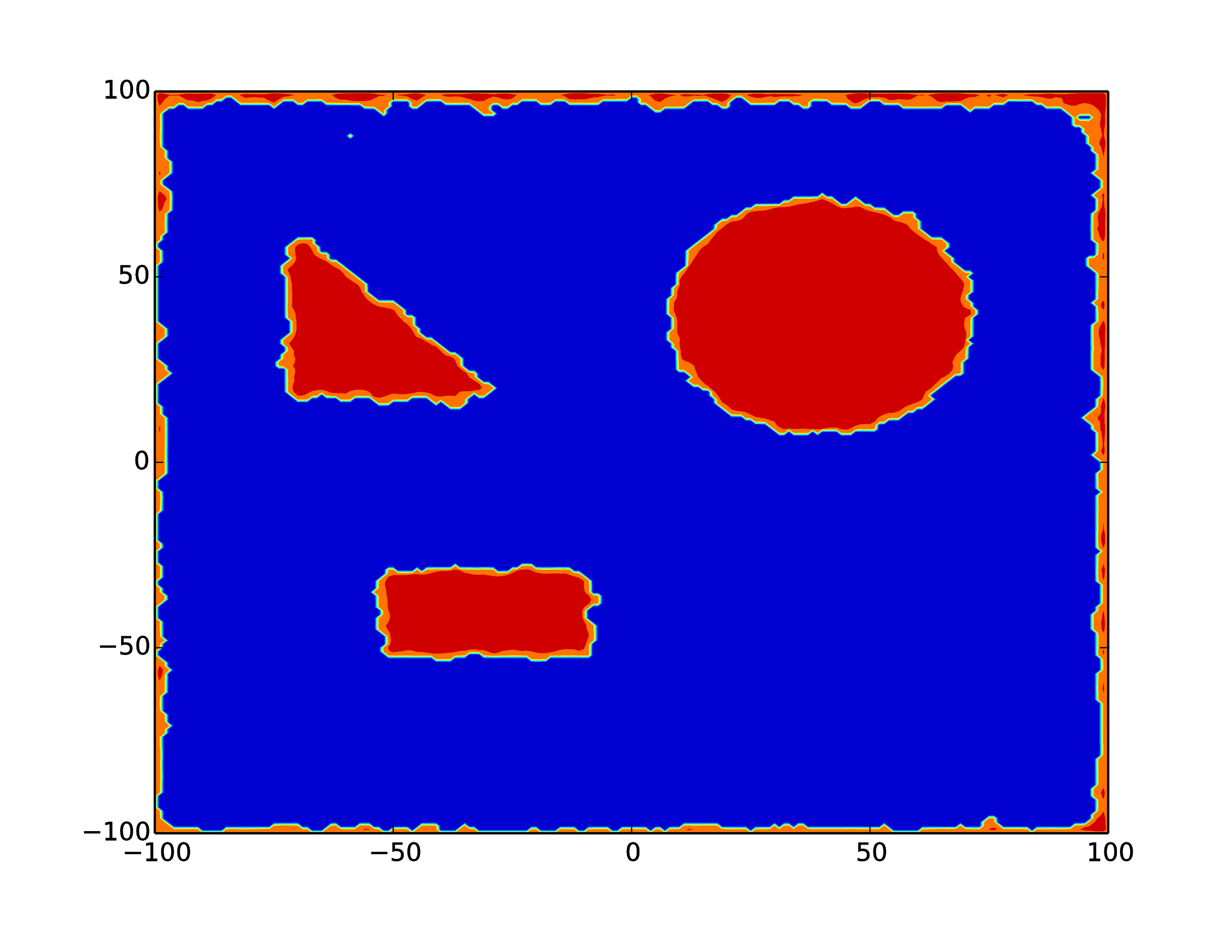
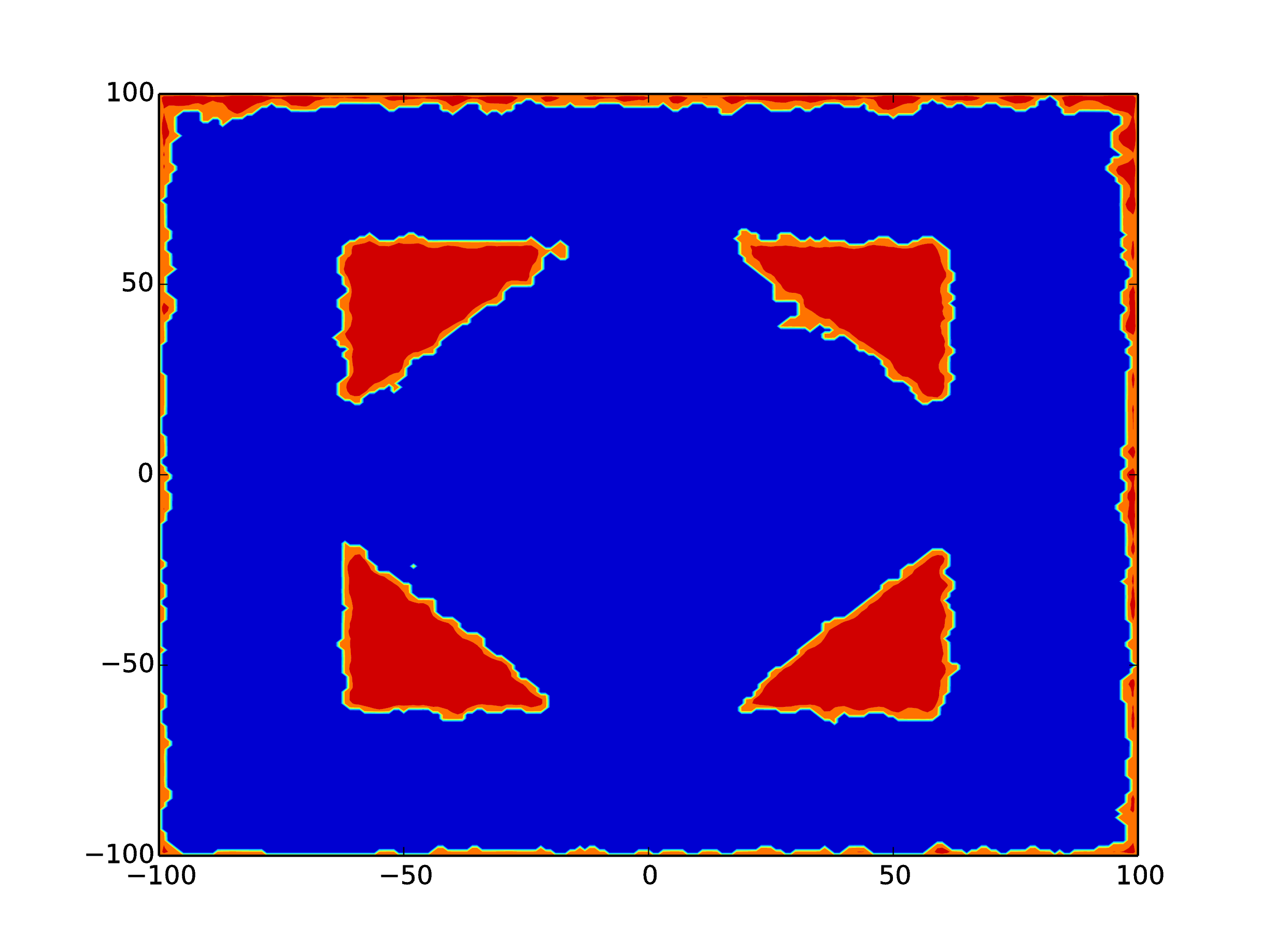
Absolute Value error
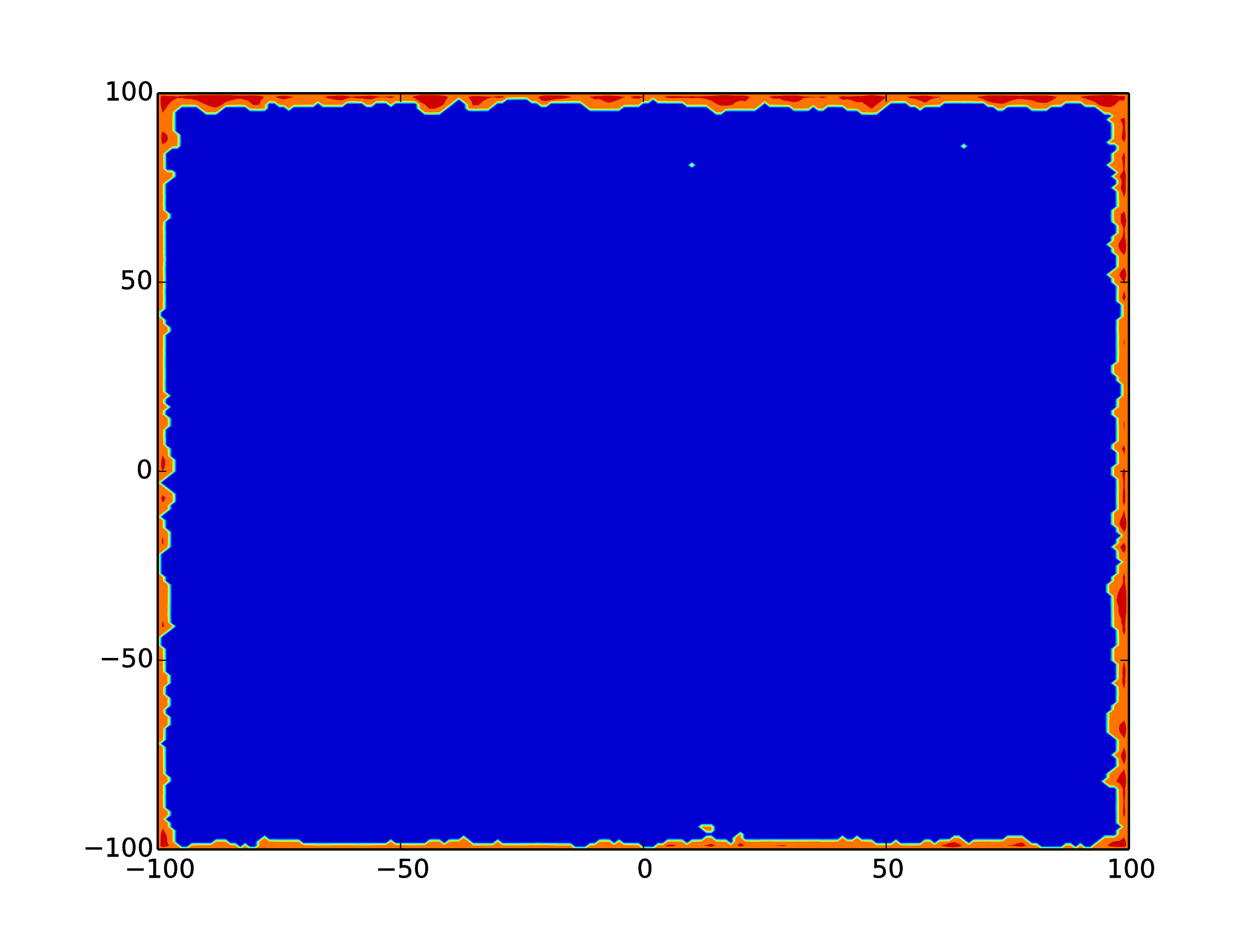
No features
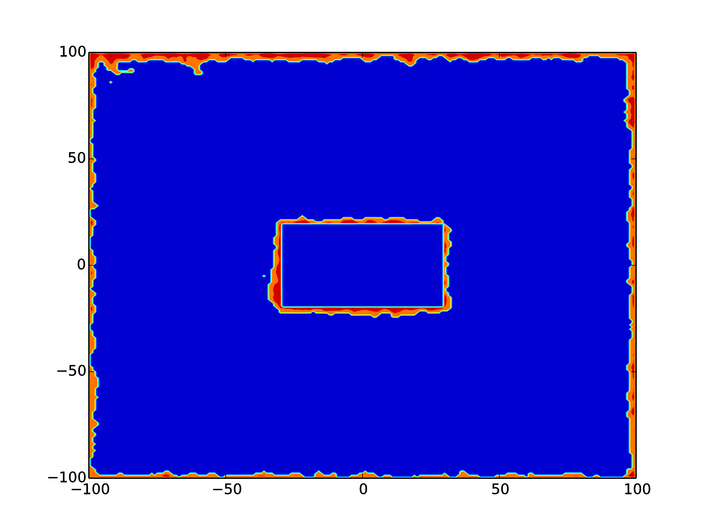
One feature
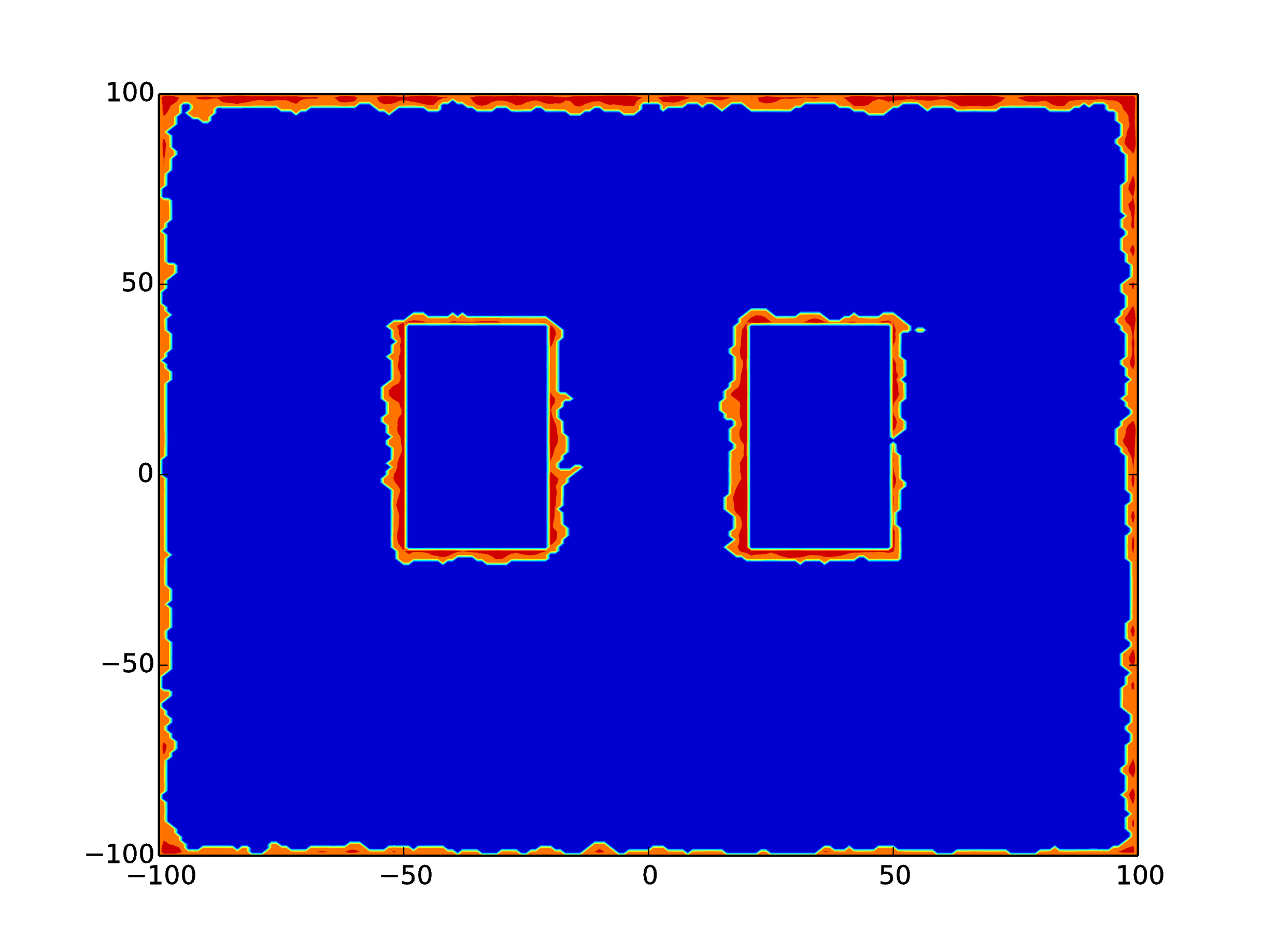
Two features
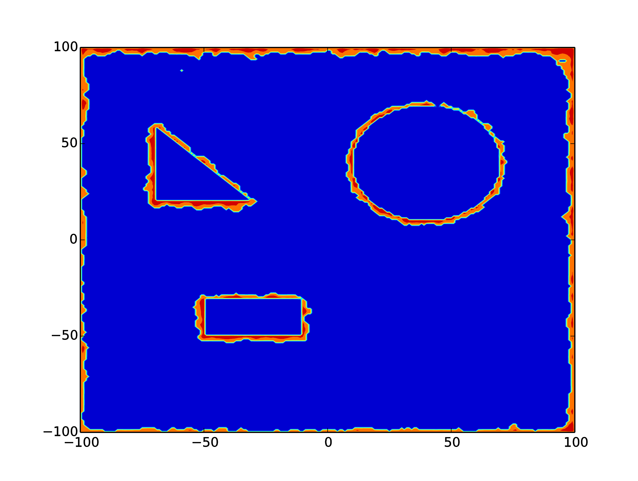
Three features
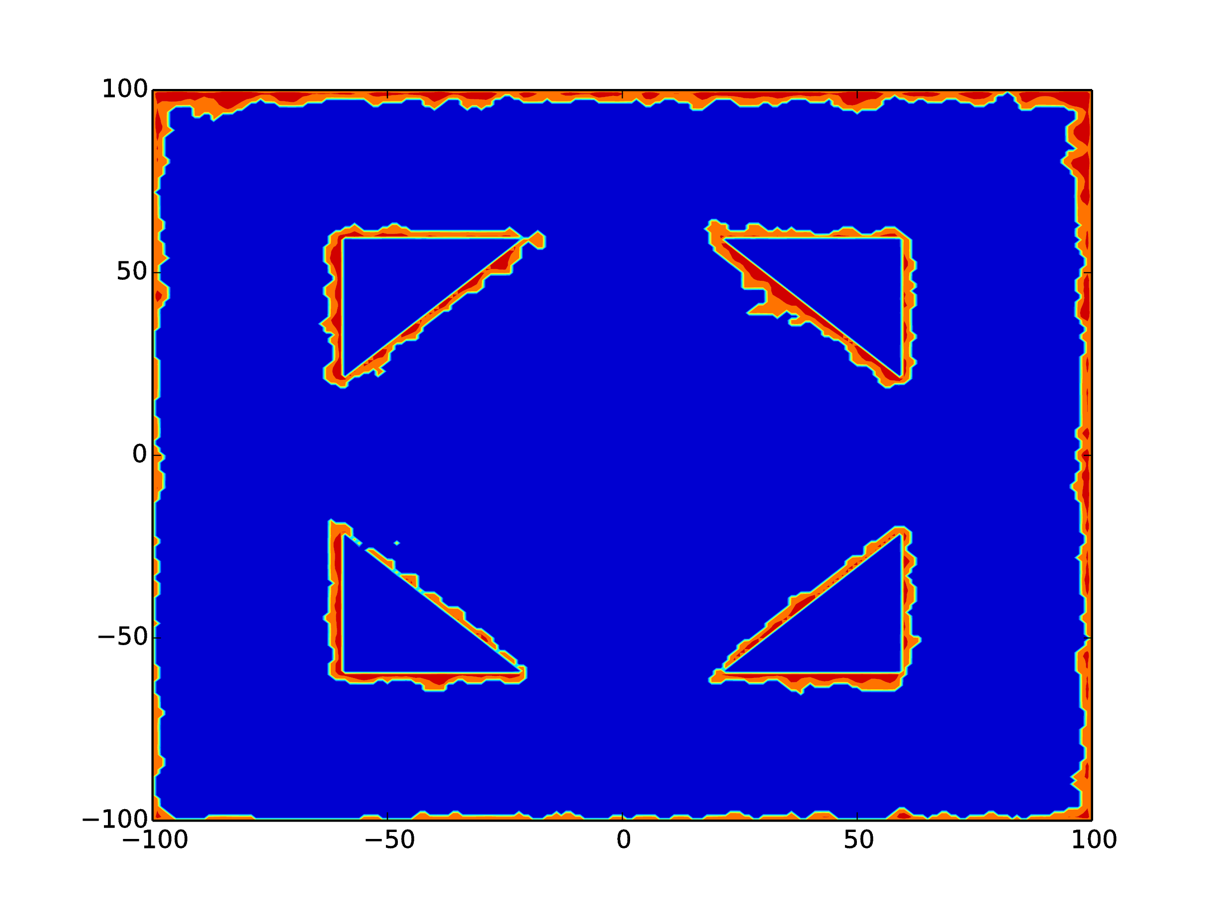
Four features
Large Complex domain
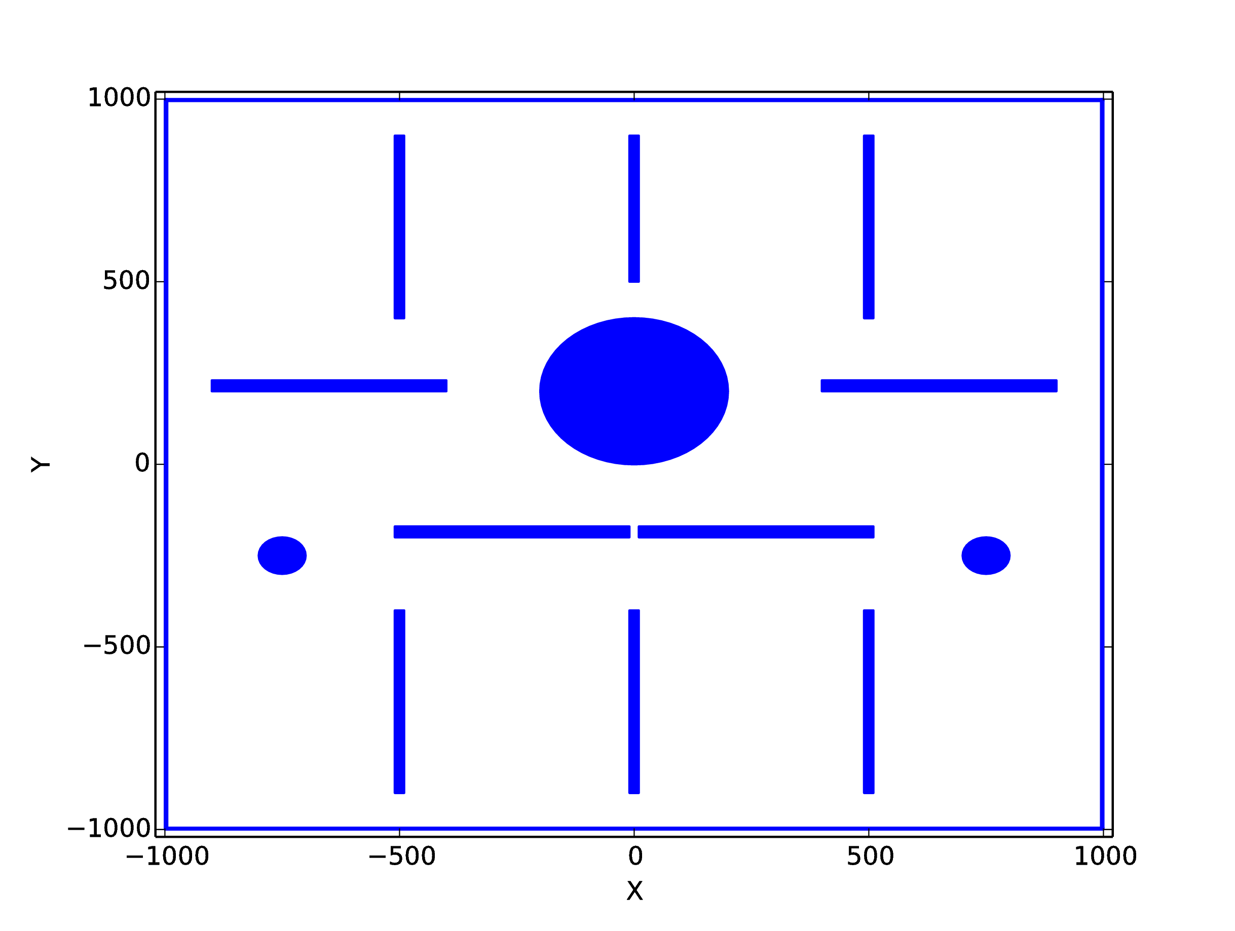
Domain
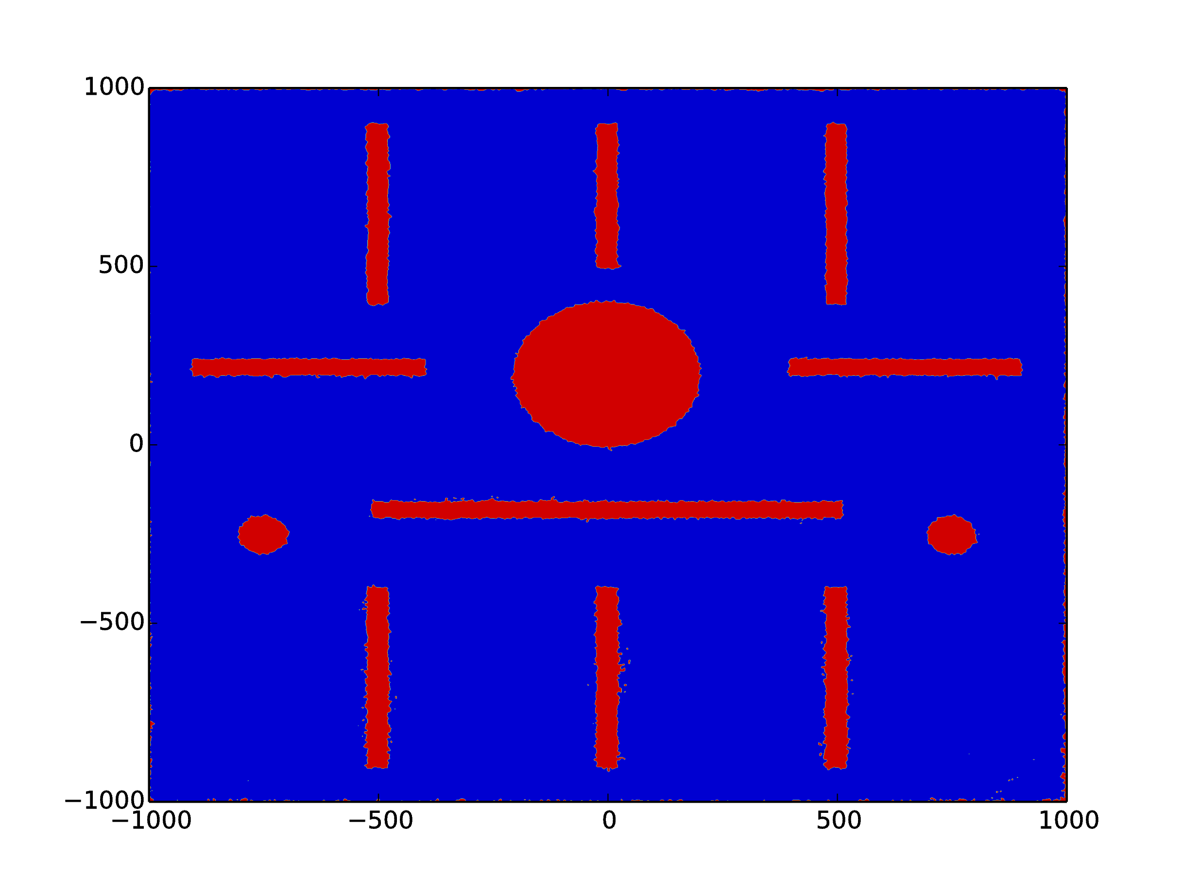
Map
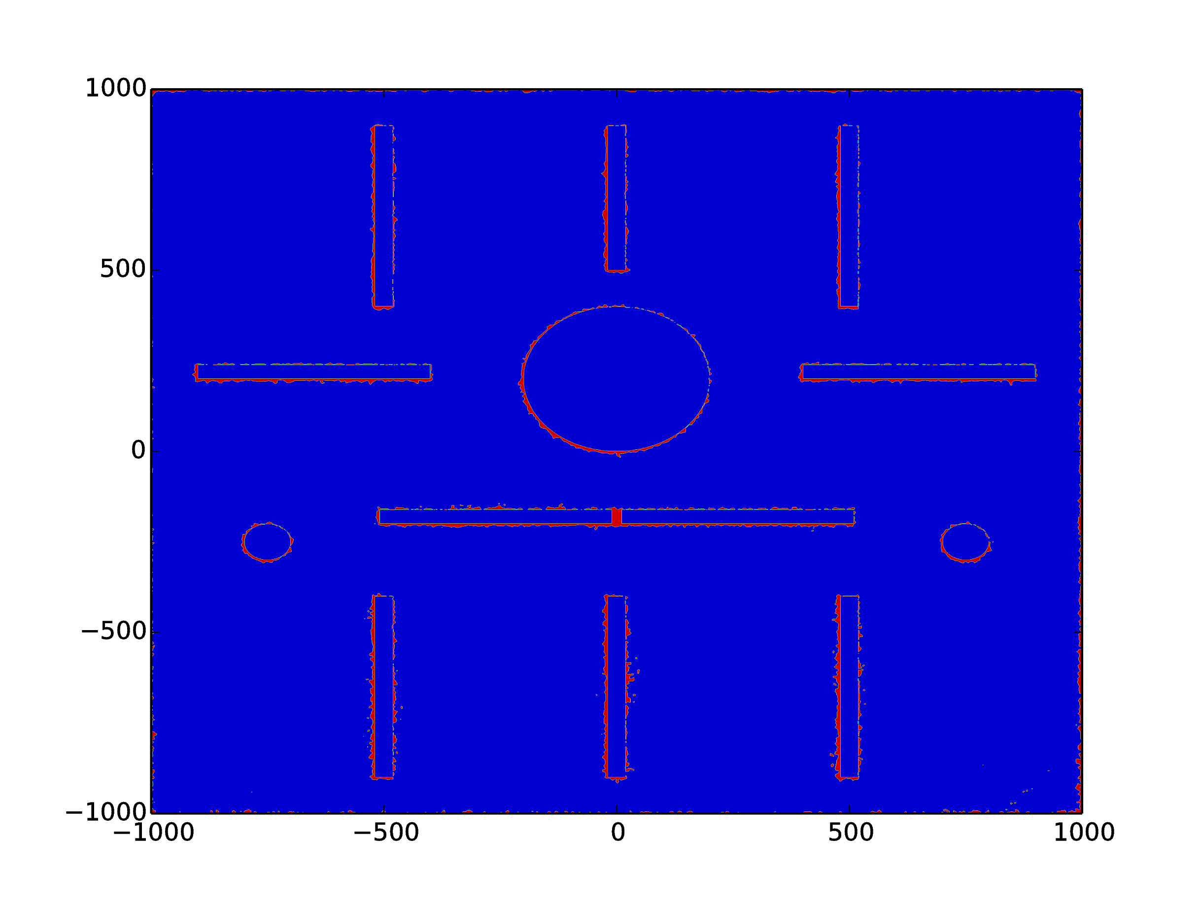
Absolute Value of error
Complex domain of size $20 m \times 20 m$, in which $N = 200$ robots were deployed for $T = 1200 s$
Effect of varying time of deployment
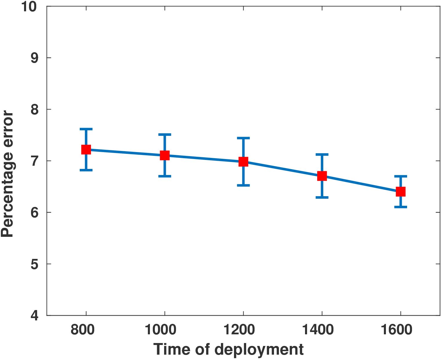
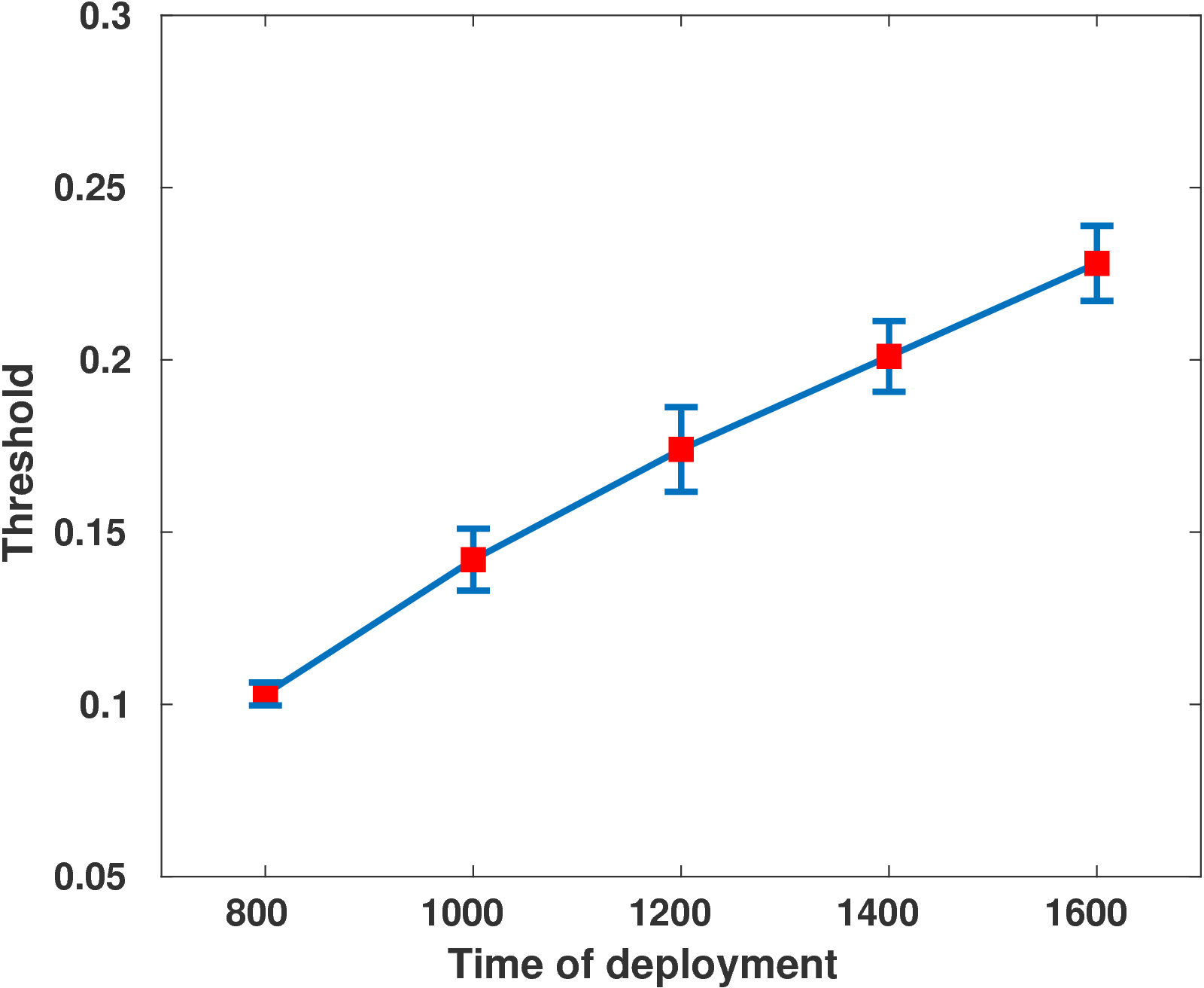
50 trails for each time of deployment.
Effect of varying number of robots
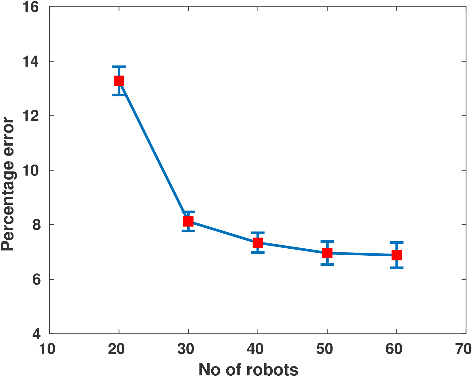
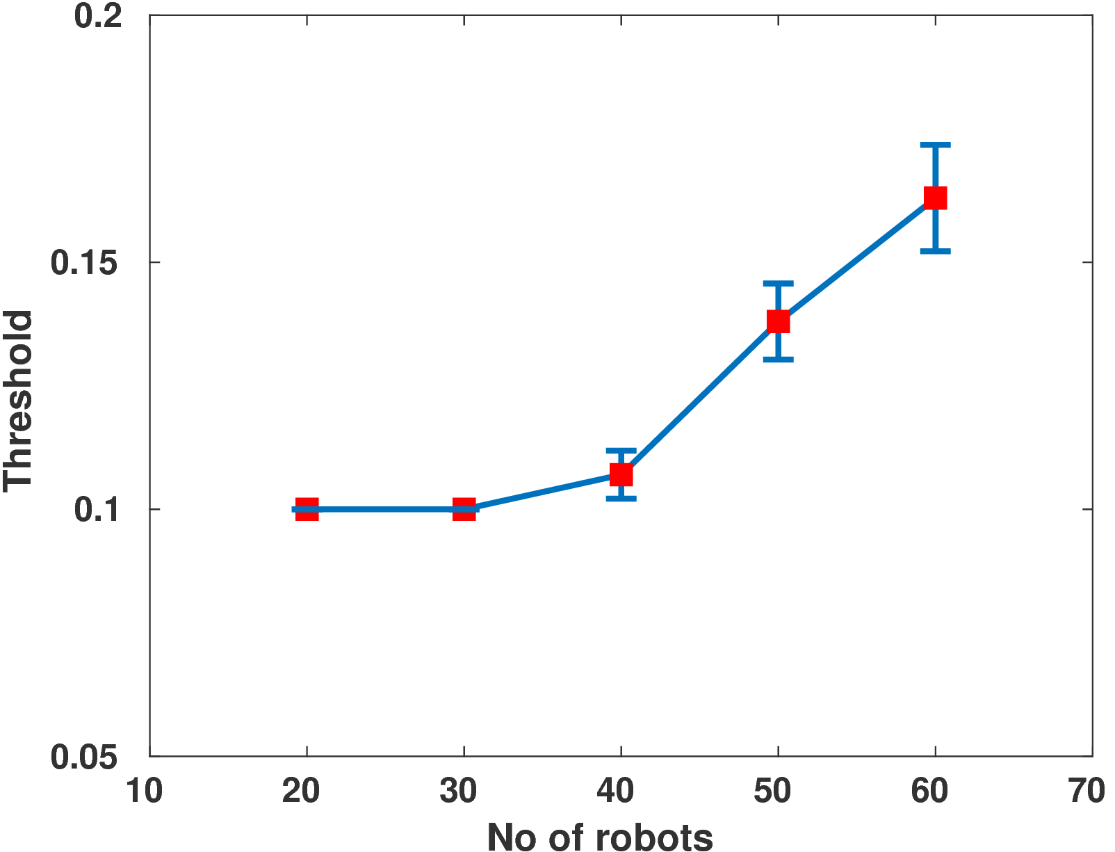
50 trails for each number of robots.
Information correlated Lévy walk exploration and distributed mapping using a swarm of robots*
*Ragesh K. Ramachandran, Zahi Kakish, and Spring Berman. Information correlated lévy walk exploration and distributed mapping using a swarm of robots. In preparation for IEEE Transactions on Robotics, 2018.
Problem Statement
We consider the problem of distributed mapping of a bounded, unknown, 2D environment using a swarm of N robots with localization capabilities.
We also formulate an information theoretic approach for exploring an unknown environment using the robotic swarm.
Information correlated Lévy walk exploration
An exploration strategy which combines information theoretic ideas with Lévy walks
Rather than moving in random directions as in Lévy walk direct the robots in direction with maximum information gain.
We use Mutual information between the distance measurement and estimated map as the metric to measure information gain.
Mutual information based direction
At time $\tau$ robot $R^i$ decides on its velocity $\mathbf{v}^i_\tau$ which it would follow for a time interval $T^i_\tau$, by solving the following optimization problem:
$$^{*}\mathbf{V}^i_{\mathbf{t}(i)} = \underset{\left \|\mathbf{v}^i_\tau \right \|=s^i, \angle \mathbf{v}^i_\tau \in[-\pi, \pi]}{arg\ \max} \frac{\mathbf{I}[\mathbf{M^i}; \mathbf{Z^i_{\mathbf{t}(i)}}\ |\ \mathbf{X^i_{\mathbf{t}(i)}}]}{C(\mathbf{V^i}_{\mathbf{t}(i)})}$$Mutual information computation for a single laser beam
$$\mathbf{I}[\mathbf{c}^{i,a}; z^{i,a}_{\tau}] = -\int_{ z^{i,a}_{\tau}}\mathbb{P}(z)\log( \mathbb{P}(z)) dz + \mathbf{K}$$ $\mathbf{c}^{i,a}$ is the set of grid cells intersected by the beam $z^{i,a}_{\tau}$. The constant $\mathbf{K}$ evaluates to $-\log(\sqrt{2\pi}\sigma) -0.5$. $\mathbb{P}(z)$ is based on the range sensor model.Distributed mapping
The robots explore the unknown domain using our exploration strategy.
Simultaneously, each robot updates its occupancy grid map based on its laser range sensor measurements.
The robots' also update their map based on the map information from their neighbors.
Consensus Protocol
$$ \mathbb{P}_{m^i_j}(k + 1) = \prod_{\hat{n} \in \mathbb{N}^i_{k} \cup i}\left( \mathbb{P}_{m^{\hat{n}}_j}(k) \right)^{a_{i,\hat{n}}(k)} \times u_m(m^i_j, \mathbf{x}^i_k,\mathbf{z}^i_k )$$ $\mathbb{P}_{m^{\hat{n}}_j}(k) $ is occupancy probability of grid cell $m^i_j$. $\mathbb{N}^i_{k}$ neighbors of robot $i$ at time step $k$. $a_{i,\hat{n}}(k)$ weights for the protocolConvergence of the protocol
Theorem: If each robot updates its occupancy grid according to the previous equation then under certain assumptions yeilds
$$\lim_{k \rightarrow \infty} \mathbb{P}_{m^i_j}[k] = <\mathbb{P}_{m_j}[0]>_{gm} \cdot \prod_{d \in \mathbf{d}} <\mathbf{u}_j[d]>_{gm}$$ Where $<\cdot>_{gm}$ is the geometric mean of the elements in a vector. $\mathbf{u}_j[d]$ is a vector of updates on $m^i_j$ based on all the measurements at time step $d$.Simulation Video
Simulation Results
Environments
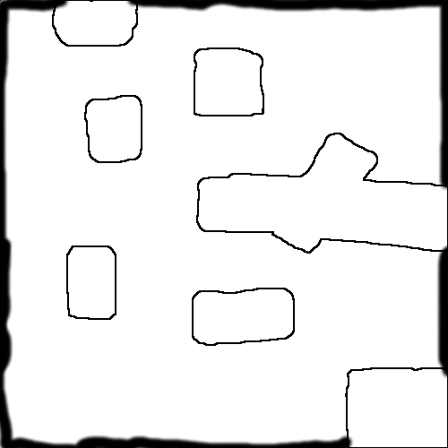

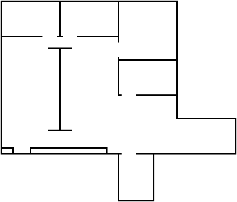
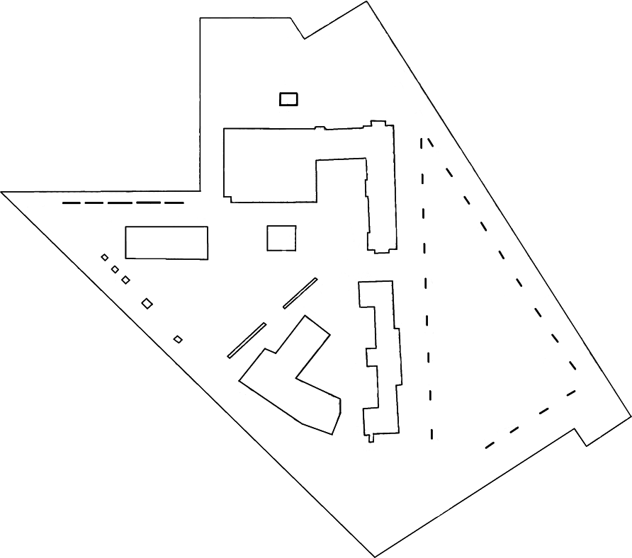
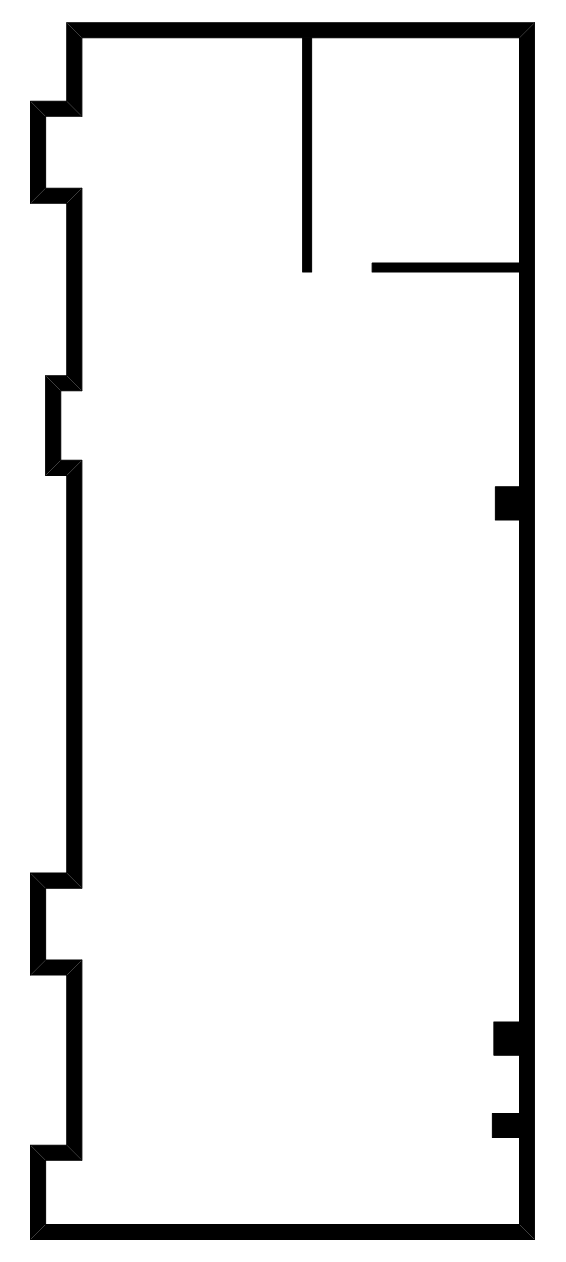
Maps
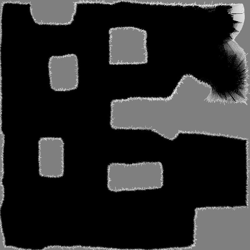
Cave

Plain
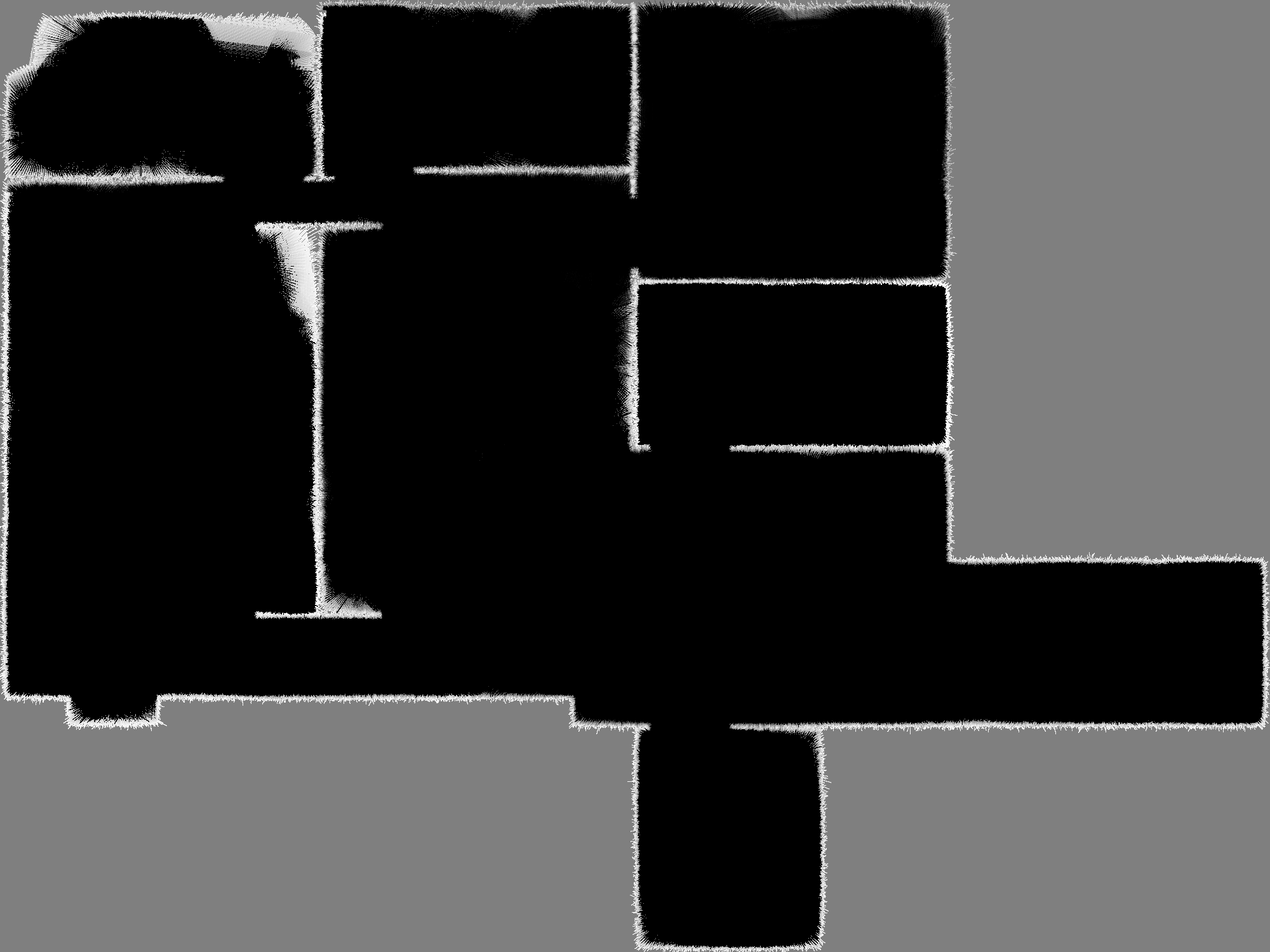
Floor Plan

University of Frieburg

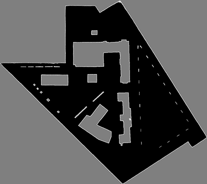
Robotics lab
Consensus in the maps of various robots
Robot 1

Robot 4

Robot 8

Robot 9

Robot 12

Robot 14

Robot 37

Robot 45
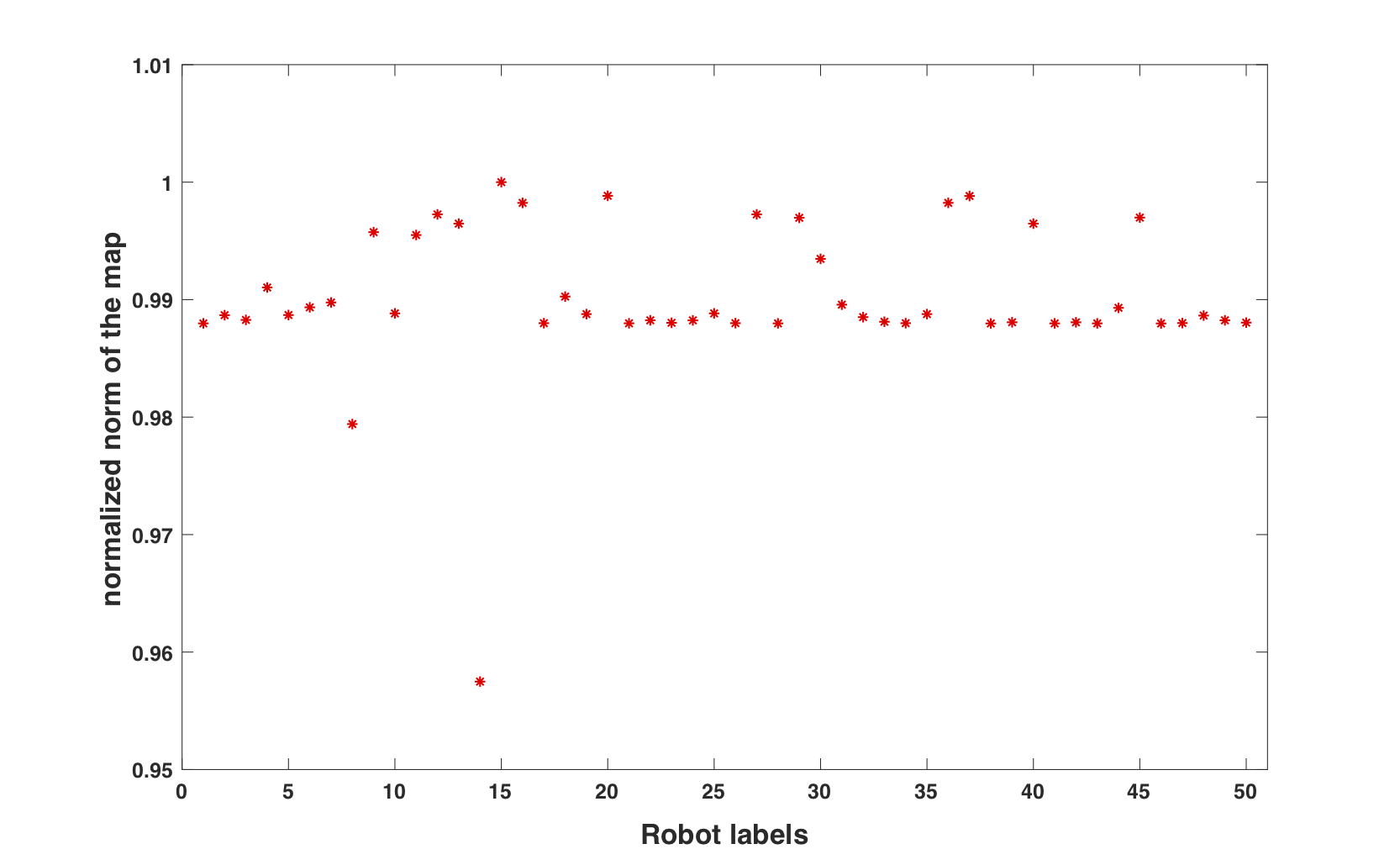
Consensus over the occupancy grid maps by 50 robots
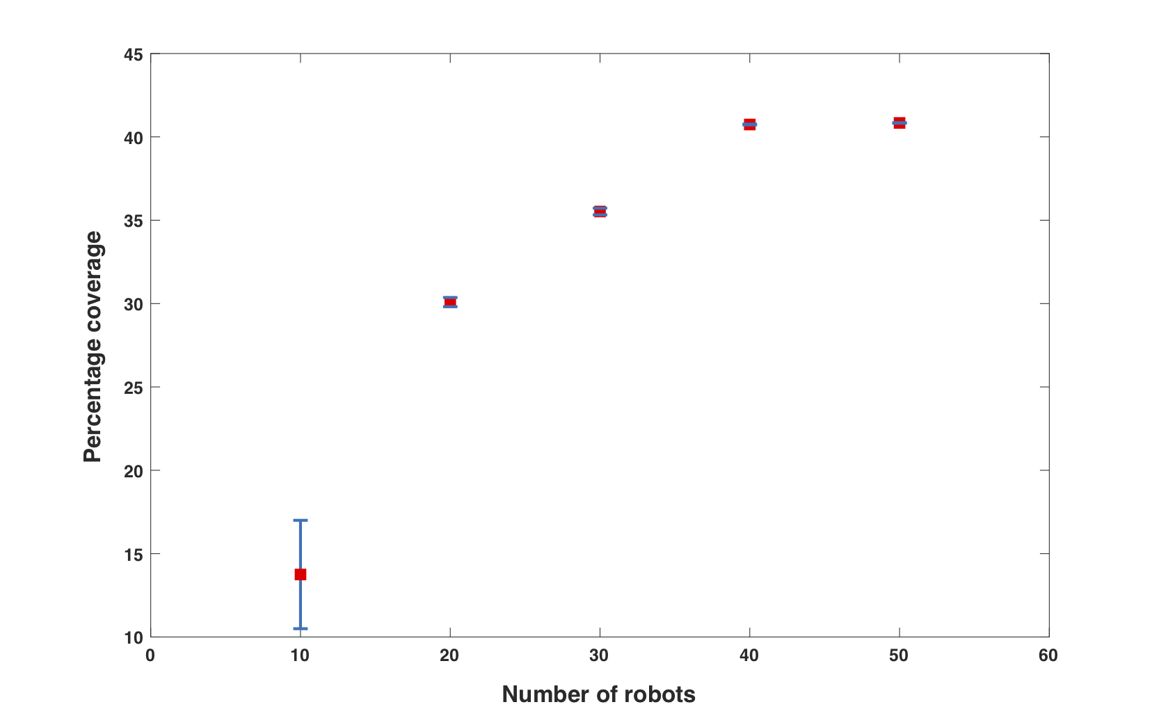
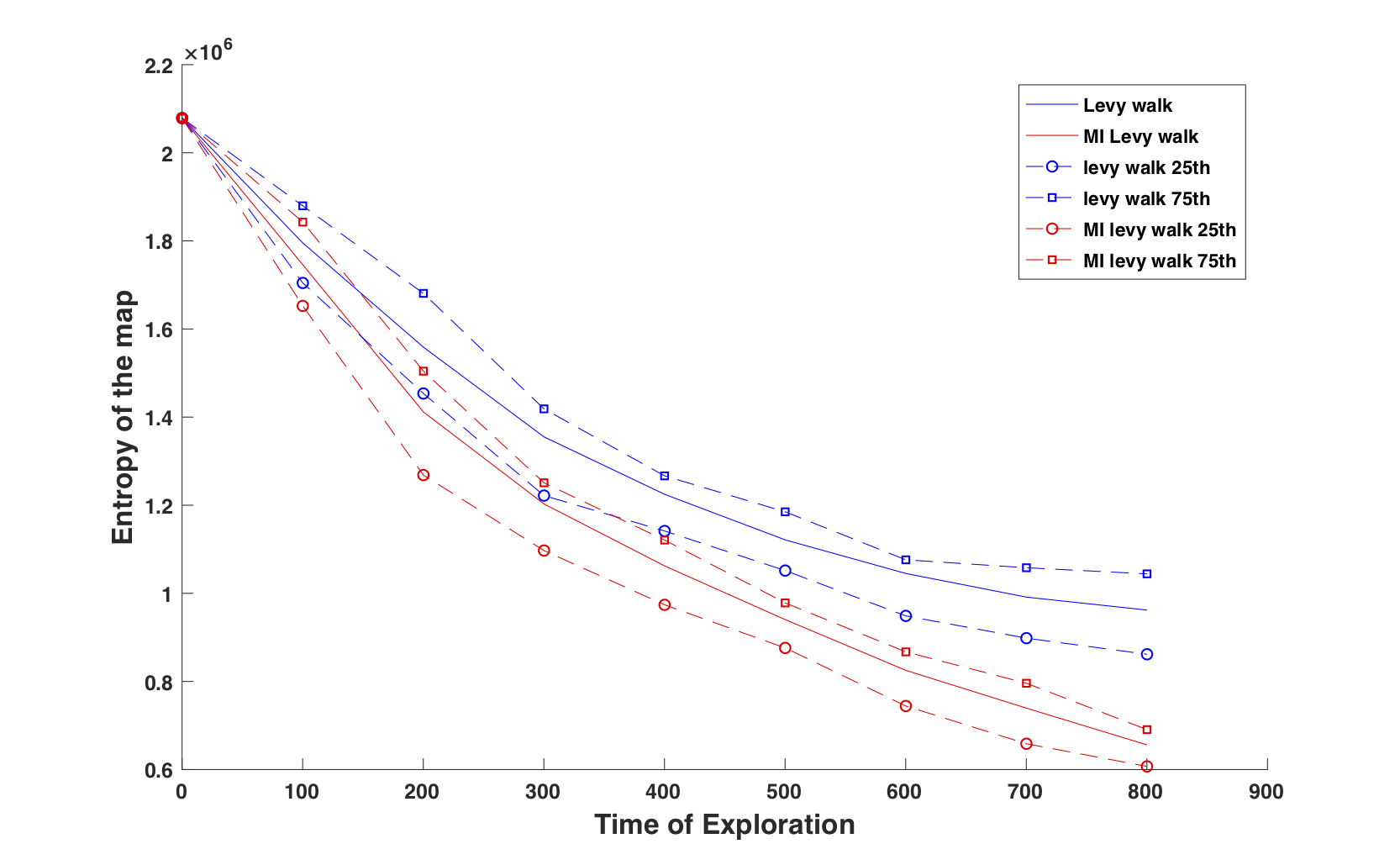
The effect of size of swarm robots on covering domain
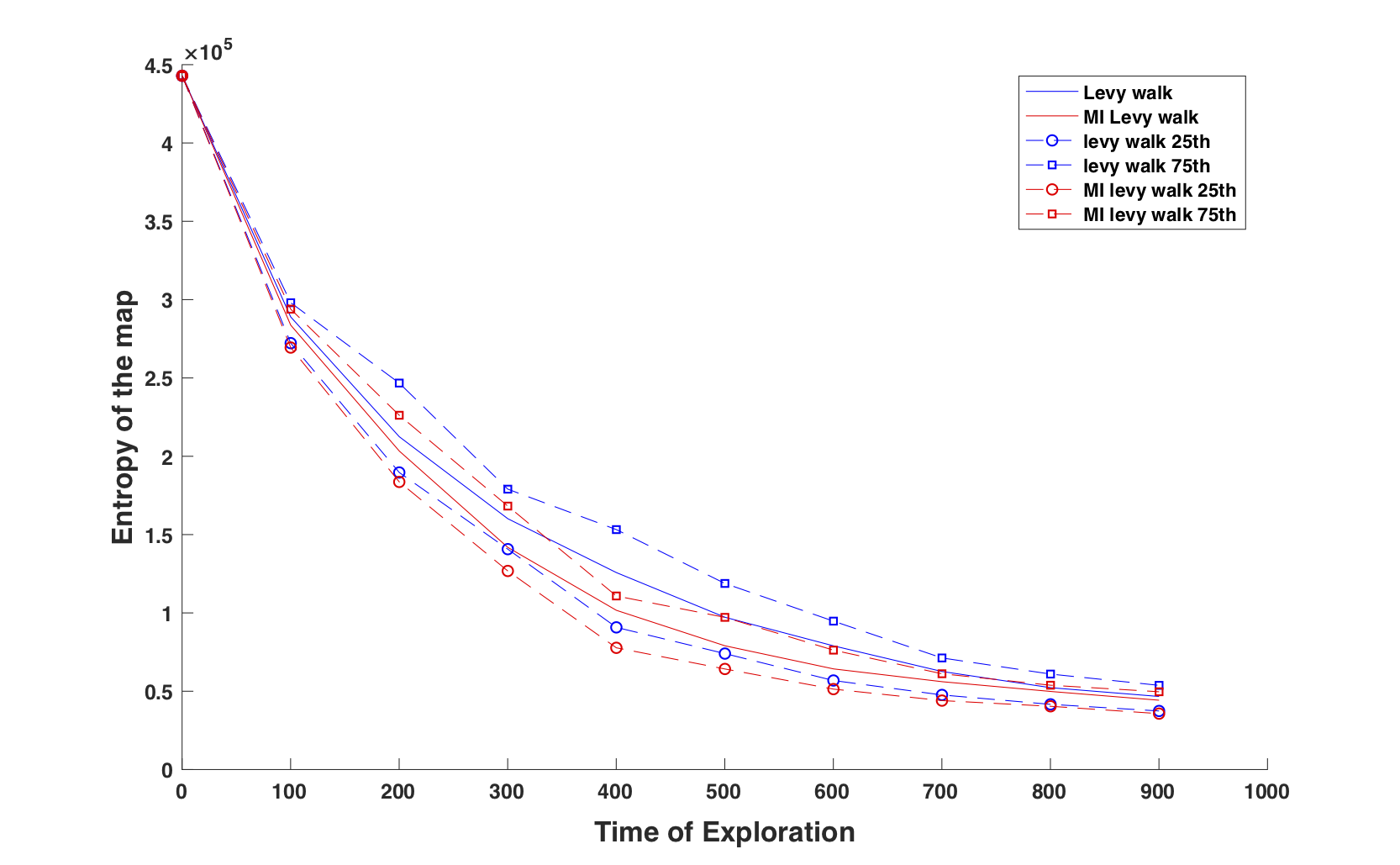
Entropy

Coverage
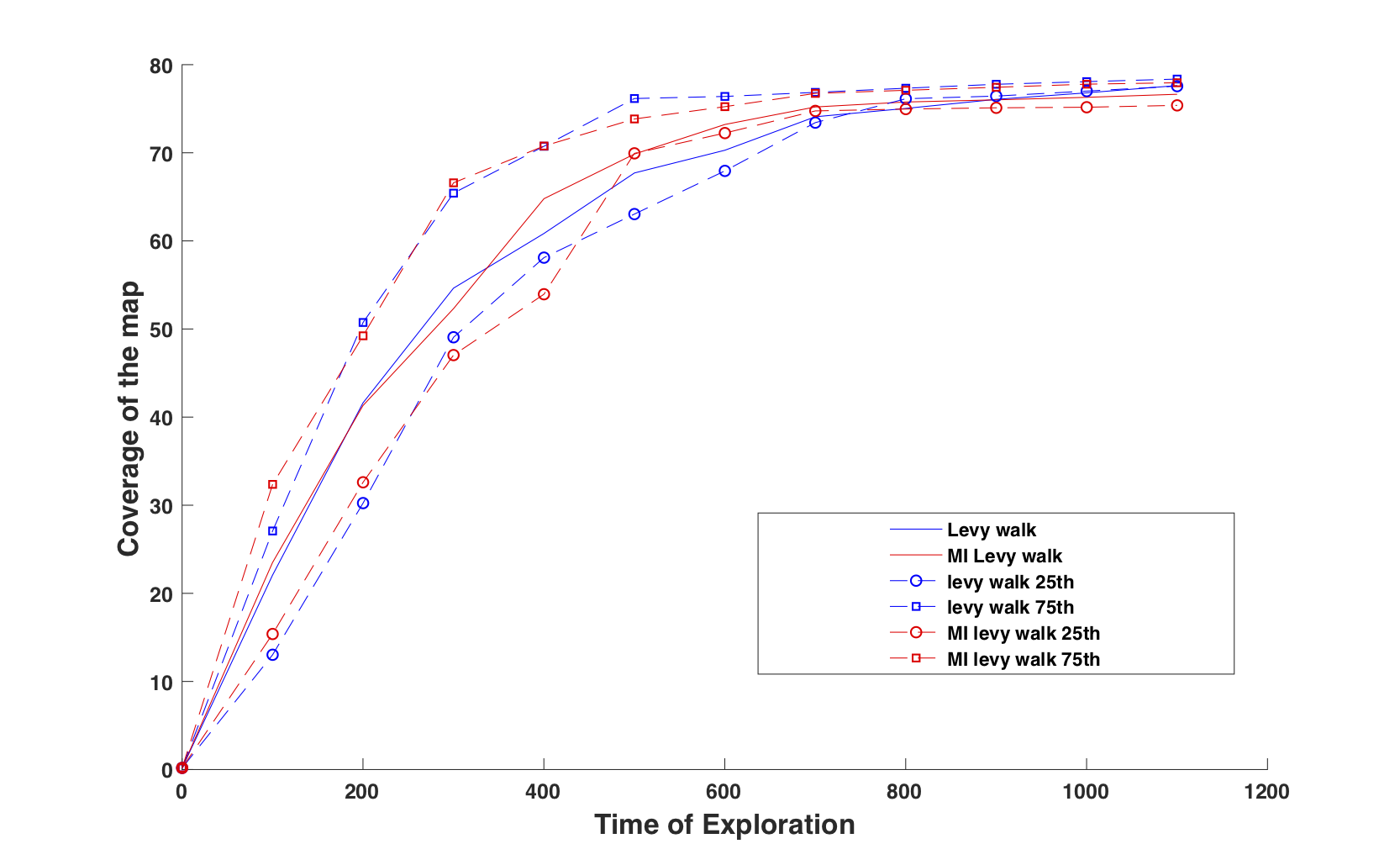
Cave
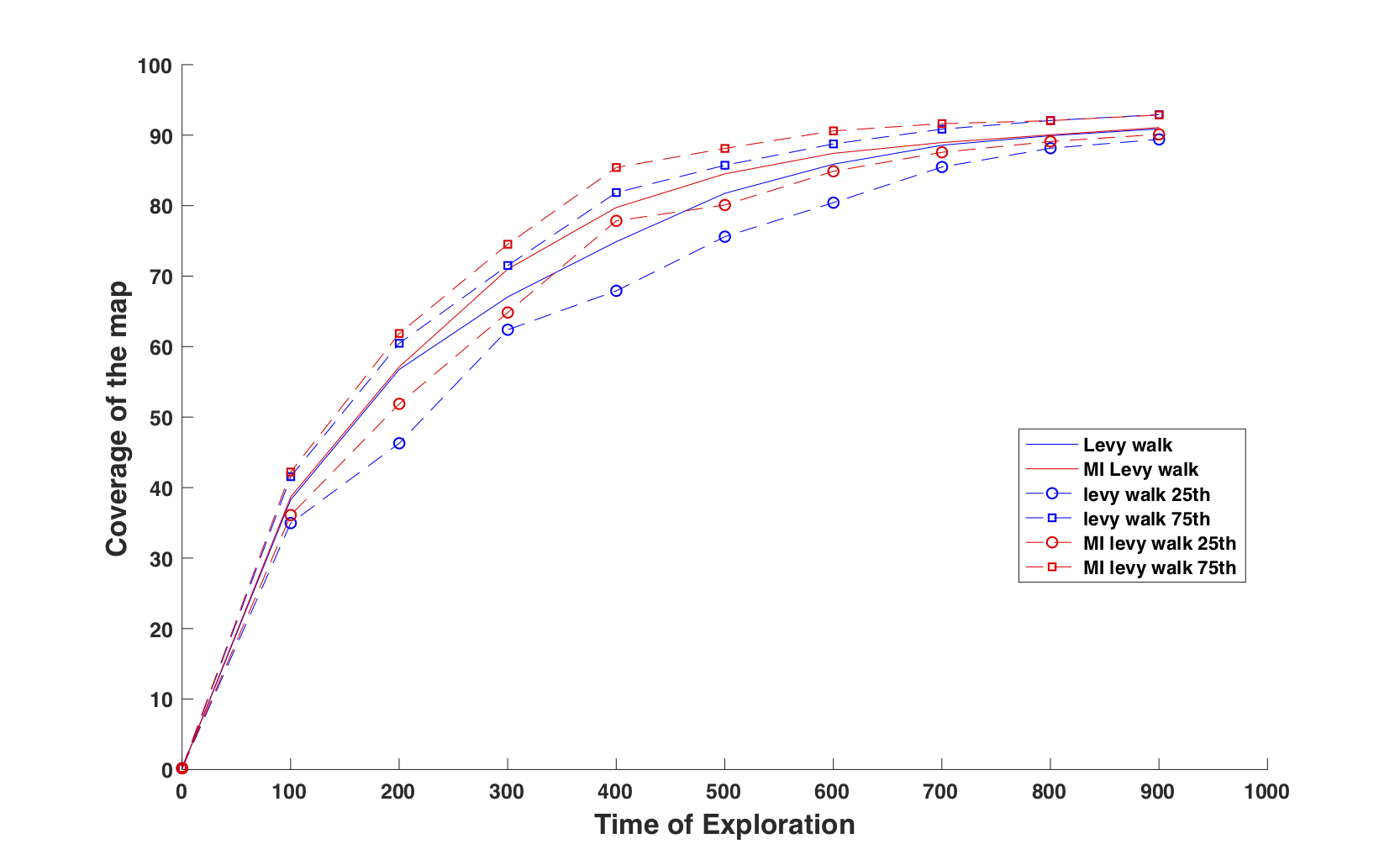
Plain
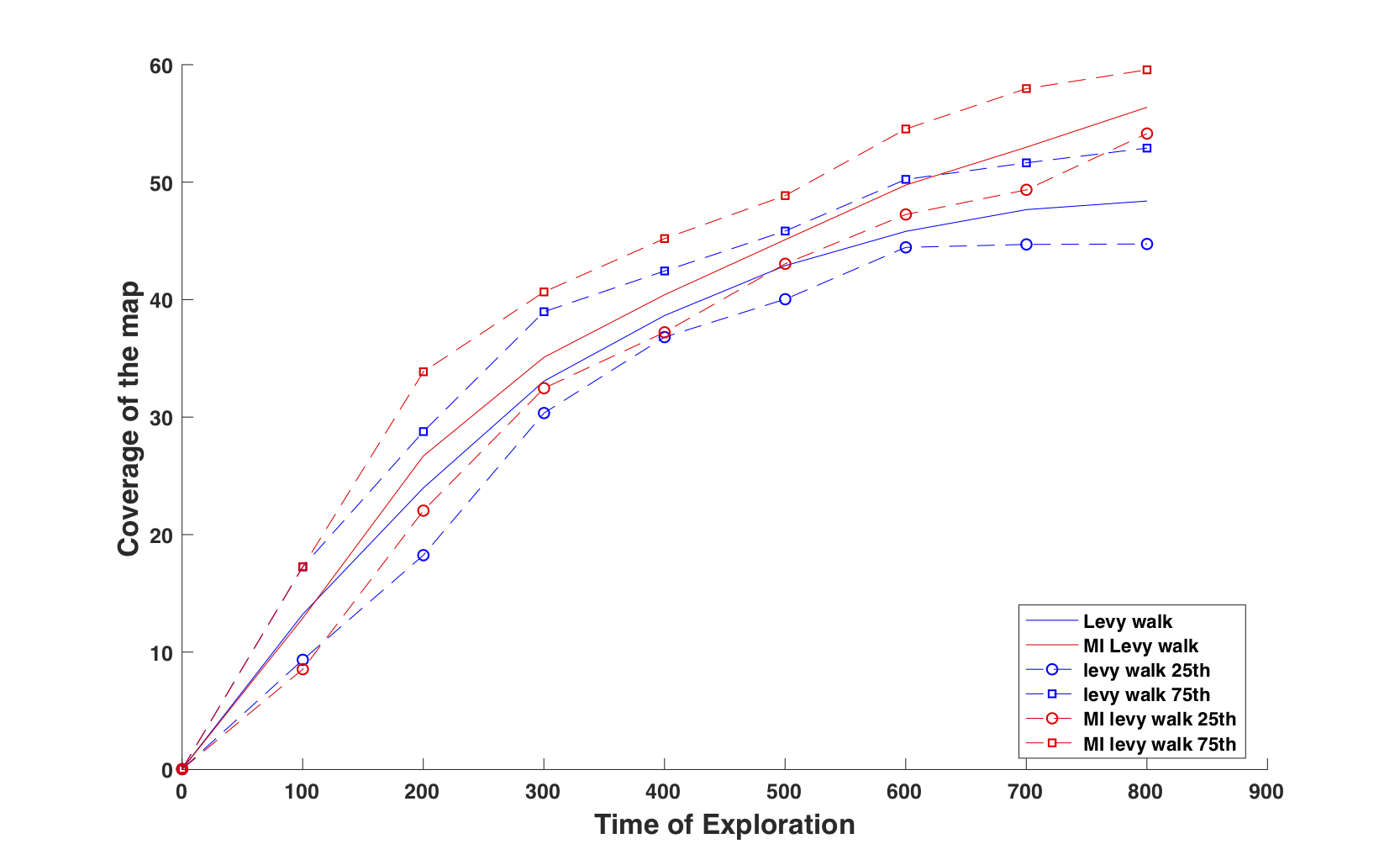
Floor Plan
Experiment Video
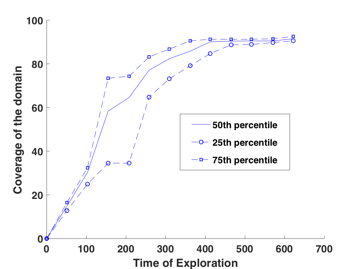
Coverage
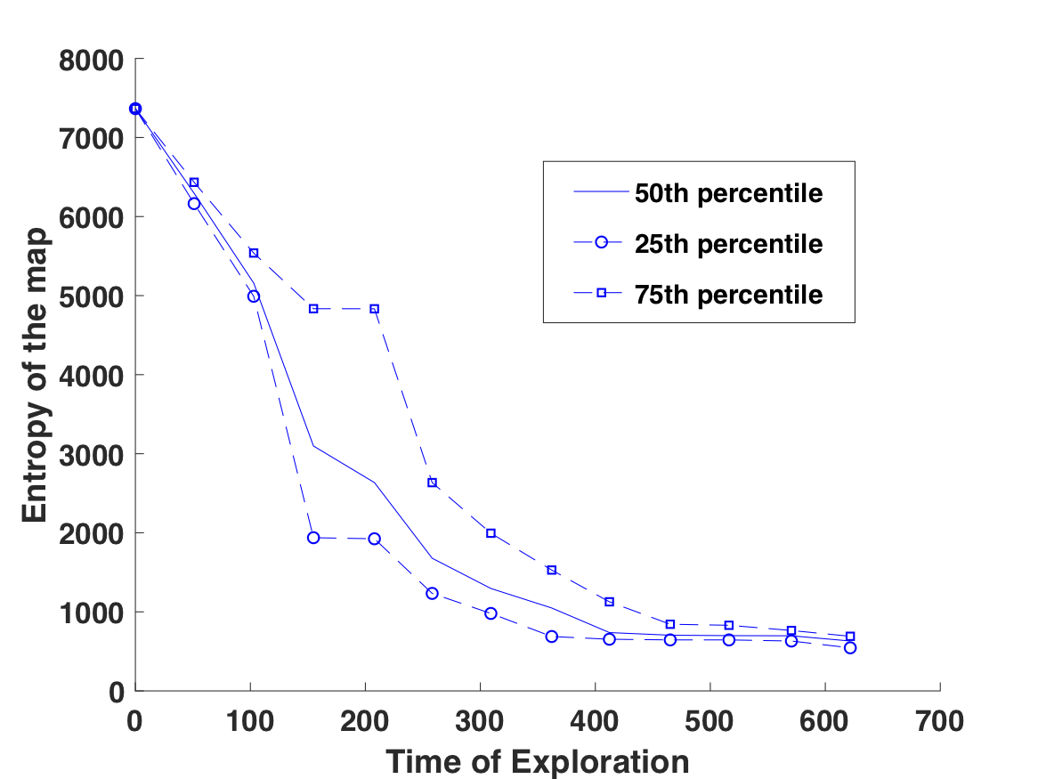
Entropy
Scalar Field Estimation by Large Networks with Partially Accessible Measurements*
*Ragesh K. Ramachandran and Spring Berman. The effect of communication topology on scalar field estimation by large networks with partially accessible measurements. In Proceedings of the 2017 American Control Conference (ACC), Seattle, WA, USA, May 24–26, 2017.
Problem Statement
We consider the problem of reconstructing a two-dimensional scalar field using measurements from a subset of a network with local communication between nodes.
The main focus of the research is a derivation of bounds on the trace of the observability Gramian of the system, which can be used to quantify and compare the field estimation capabilities of chain and grid networks.
A comparison based on a performance measure related to the $H^2$ norm of the system is also used to study the robustness of the network topologies.
Motivation & Related work
Solution to estimation problem is associated with the observability of the system.
Little work on estimation of initial conditions other than through the inversion of the observability Gramian
Checking the rank condition for large interconnected systems is computationally ill-conditioned due to the high dimensionality of the observability Gramian.
A graph-theoretic characterization of observability has been more widely used than a matrix-theoretic characterization for large complex networked systems.
The observability of complex networks is studied in Yang-Yu Liu et al.(2013) using structural observability, which presents a general result that holds true for most of the chosen network parameters (the edge weights).
In Meng Ji et al.(2007), a graph-theoretic approach based on equitable partitions of graphs is used to derive necessary conditions for observability of networks
Alternately, Zhengzhong Yuan et al.(2013) uses a matrix-theoretic approach to develop a maximum multiplicity theory to characterize the exact controllability of a network based on the network spectrum.
Problem Statement
Consider a set of N nodes with local communication ranges and local sensing capabilities.
Each node is capable of measuring the value of a scalar field at its location and communicating this value to its neighbors
The nodes take measurements at some initial time and transmit this information using a nearest-neighbor averaging rule
The problem is to reconstruct the initial measurements taken by all the nodes from the measurements of a subset of accessible nodes.
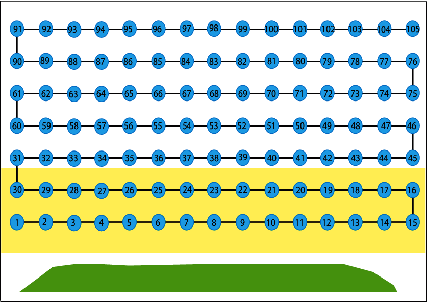
Chain topology
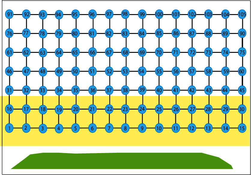
Grid topology
Illustration of the chain and grid network topologies. The blue circles are nodes and are labeled by numbers. Nodes in the yellow region are accessible nodes.
System dynamics
We define the information flow dynamics of node $i$ as: $$\frac{dx_i}{dt} = \sum_{(i, j) \in \mathcal{N}_i } (x_j-x_i)$$ $\mathcal{N}_i$ denote the set of neighbors of node $i$.
The information flow dynamics over the entire network becomes : $$\dot{\mathbf{X}}(t) = - \mathbf{L}(\mathcal{G}) \mathbf{X}(t), \mathbf{Y}(t) = \mathbf{C} \mathbf{X}(t)$$ $$\mathbf{X}(0) = \mathbf{X}_0.$$ $\mathbf{L}(\mathcal{G})$ denote the Laplacian of the graph. $\mathbf{Y}(t)$ is the measurement vector at time $t$.
Scalar Field Reconstruction
We solve the scalar field reconstruction problem by posing it as an optimization problem. We frame our optimization objective as the computation of $ \mathbf{X}_0$ that minimizes the functional $J(\mathbf{X}_0)$, defined as :
$$J(\mathbf{X}_0) = \frac{1}{2}\int_{0}^{T}\left \| \mathbf{Y}(t) - \hat{\mathbf{Y}}(t) \right \|_2^2 dt + \frac{\lambda}{2}\left \| \mathbf{X}_0 \right \|^2$$subject to the constraint of the system dynamics. $\hat{\mathbf{Y}}(t)$ is the observed data.
The convexity of $J(\mathbf{X}_0)$ ensures the convergence of gradient descent methods to its global minima.
Gradient Computation
The gradient can be computed as :
$$\delta J(\mathbf{X}_0) = P(T) + \lambda \mathbf{X}_0$$We find $P(T)$ by solving following equation forward :
$$\frac{dP}{d\tau} = - \mathbf{L}^*(\mathcal{G})P(\tau) + \mathbf{C}^*\hat{u}(\tau), ~~~P(0) = 0$$Where $\hat{u}(\tau) \equiv \mathbf{Y}(T - \tau) - \hat{\mathbf{Y}}(T - \tau)$
$\mathbf{L}^*(\mathcal{G})$ and $\mathbf{C}^*$ are transposes of $\mathbf{L}(\mathcal{G})$ and $\mathbf{C}$ respectively
Simulation: Chain Topology

Actual field
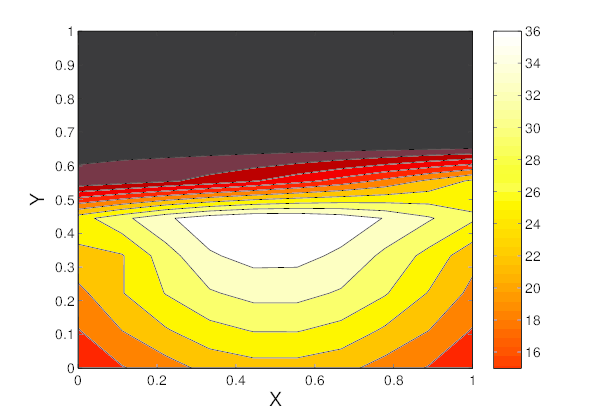
Estimated field
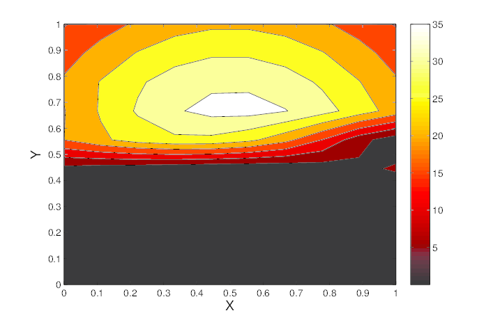
Absolute value of error
Gaussian function estimation using 100 nodes with a chain communication topology. Temporal data is acquired from 30 nodes over a time period of 50 sec.
Simulation: Grid Topology
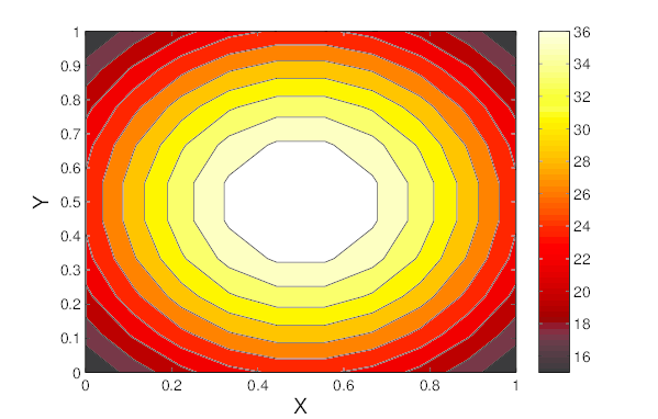
Actual field
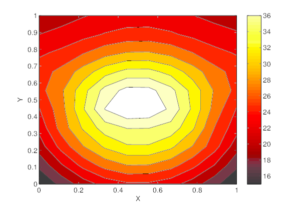
Estimated field
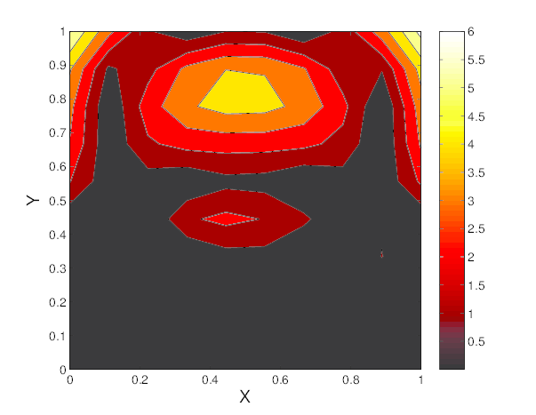
Absolute value of error
Gaussian function estimation using 100 nodes with a grid communication topology. Temporal data is acquired from 30 nodes over a time period of 50 sec.
Simulation Using Ocean Salinity Data
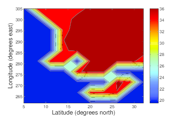
Actual salinity field
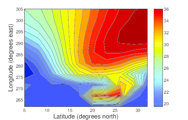
Estimated salinity field
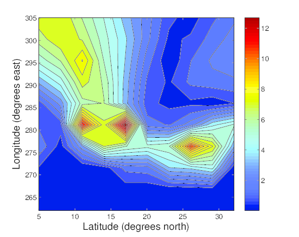
Absolute value of error
Estimation of salinity (psu) over a section of the Atlantic Ocean at a depth of $25$ m. The network consists of 100 nodes with a grid communication topology. Temporal data is acquired from 30 nodes over a time period of 50 sec.
Effect Of Network Topology On Estimation Performance
Comparing the chain and grid results, it is evident that there is some fundamental limitation arising from the network structure which makes the system with the chain topology practically unobservable.
Degree of observability is used as a metric to study effect of network structure.
Commonly used measures of the degree of observability (controllability) are the smallest eigenvalue, the trace, the determinant, and the condition number of the observability (controllability) Gramian
For large, sparse networked systems, the Gramian can be highly ill-conditioned, which makes numerical computation of its minimum eigenvalue unstable.
We use the trace of the observability Gramian which can be interpreted as the average sensing effort required to estimate its initial state.
We compute the estimate on the trace of the observability Gramian in form of upper and lower bounds.
We compared the chain and grid topology using the bounds on the trace.
Upper And Lower Bounds On Trace Of The Observability Gramian
Theorem: Let $\mathcal{G}$ be an unweighted, undirected graph that represents the communication network of a set of $N$ nodes with information dynamics and output map. If we label $\mathit{V(\mathcal{G})} $ such that $k \leq N$ sensor nodes in $\mathit{V(\mathcal{G})} $ are labeled as $1, 2, ..., k$, then $\mathbf{C} = \left[ \mathbf{I}_{k \times k}\ \mathbf{0}_{k \times (N - k)} \right]$. Assuming that $\mathbf{L}(\mathcal{G})$ is diagonalizable and that $\lambda_1 \geq \lambda_2 \geq ... \geq \lambda_N $ are its eigenvalues, there exist real constants $c_1 \leq c_2 \leq ... \leq c_N$ such that
$$\sum_{i=1}^{k} c_i ~\leq ~Trace\left( \mathit{W}_O(0,T) \right) ~\leq~ \sum_{i=0}^{k-1} c_{N-i}$$where $c_i = \int^{T}_{0} e^{-2\lambda_i t} dt$.
Estimate the Trace For Chain And Grid
Let $\lambda_{N-i}^{c}$ and $\lambda_{N-i}^{g}$ denote the $(N-i)^{th}$ eigenvalue of $\mathbf{L}(\mathcal{G}_c)$ and $\mathbf{L}(\mathcal{G}_g)$, respectively.
Then, $\lambda_{N-i}^{c} = 4\sin^2 \left(\frac{\pi i}{2N} \right)$ and $\lambda_{N-i}^{g} = 4\sin^2 \left(\frac{\pi i}{2\sqrt{N}} \right)$ for $i \in \{0, 1, ..., k-1\}$, $k < \sqrt{N}$.
Applying the theorem, we get the upper bound on $Trace\left( \mathit{W}_O(0,T) \right)$ for the chain network as. $$T + \frac{N^2}{2\pi^2 } \left (\sum_{i=1}^{k-1}\frac{1 -e^{-2\frac{\pi^2 i^2}{N^2}T}}{i^2} \right)\ (Scales\ quadratically\ in\ N)$$
Similarly for the grid network we get, $$T + \frac{N}{2\pi^2 } \left ( \sum_{i=1}^{k-1}\frac{1 -e^{-2\frac{\pi^2 i^2}{N}T}}{i^2} \right )\ (Scales\ linearly\ in\ N)$$
Comparison of the degree of observability
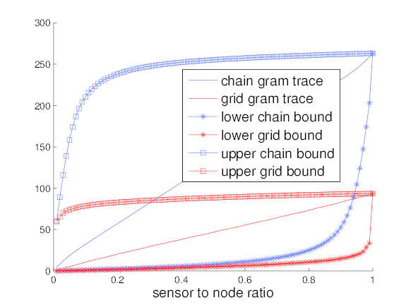
Networks with 100 nodes
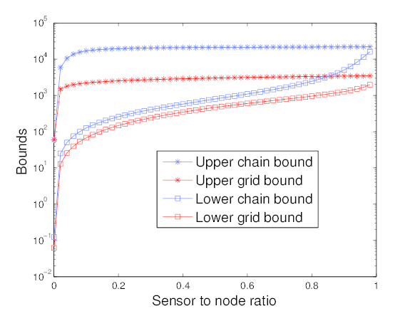
Networks with 10000 nodes
Comparison of the degree of observability based on the trace of the observability Gramian and its bounds. The trace is computed numerically using the eigenvalues of $\mathbf{L}(\mathcal{G})$.
Effect Of Network Topology On Robustness To Noise
We analyze the effect of noise on the output of first-order linear dynamics that evolve on chain and grid network topologies.
The $\mathcal{H}_2$ norm of a system gives the steady-state variance of the output when the input to the system is white noise and when the system is Hurwitz.
For unstable systems, the finite steady-state variance can be computed only when the unstable modes are unobservable from the outputs.
Consider the augmented system dynamics written as, $$\dot{\mathbf{X}}(t) = - \mathbf{L}(\mathcal{G}) \mathbf{X}(t) + \mathit{W}$$ where $\mathit{W} \in \mathbf{R}^N$ denotes a zero mean, unit covariance white noise process.
We can make the zero mode unobservable, in order to use the $\mathcal{H}_2 $ norm as a measure to quantify the effect of noise on the system output
Following the approach in Milad Siami et al.(2014) We make the zero mode unobservable by choosing the matrix $\mathbf{C}$ which annihilates the vector $\mathbf{1}_N$.
The $\mathcal{H}_2 $ norm, denoted as $\mathcal{H}_{\mathcal{K}_N} ^{(1)}(\mathbf{L}(\mathcal{G}))$, for a chosen $ \mathbf{C} $ can be defined from as $$\mathcal{H}_{\mathcal{K}_N} ^{(1)}(\mathbf{L}(\mathcal{G})) = \sum_{i = 1}^{N-1}\frac{1}{2\lambda_i}$$ where $\lambda_1 \geq \lambda_2 \geq ... \geq \lambda_N = 0 $ are the eigenvalues of $\mathbf{L}(\mathcal{G})$.
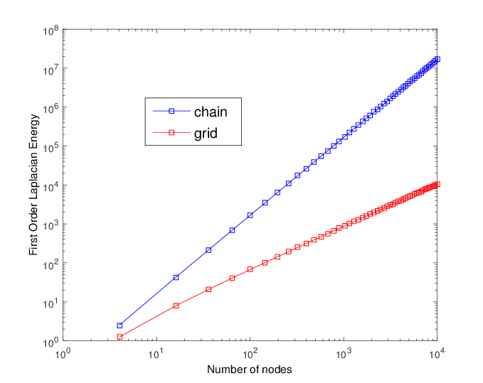
First order Laplacian energy
Future work
Experimental Validation of Reaction-Based Mapping with Nanoparticle Swarms
Extending the network theory work for network topology estimation using ideas from information geometry.
Distributed Multi Target Tracking based on random finite sets.
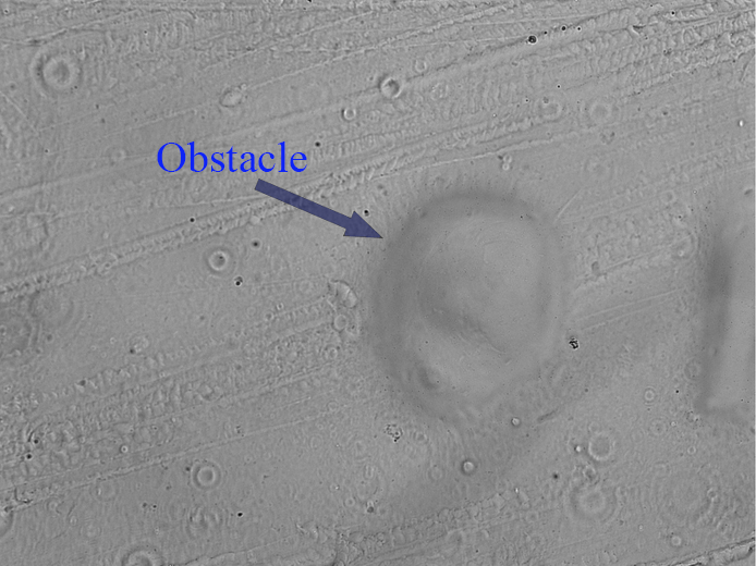
Circular obstacle
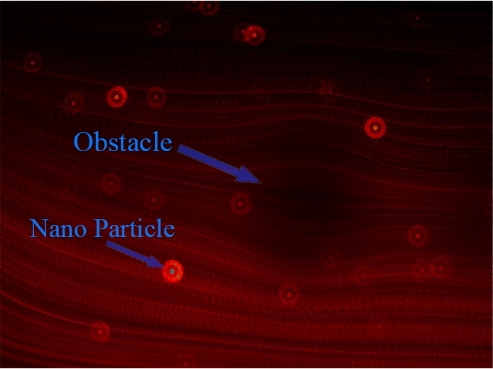
Nanoparticles near the circular obstacle
Grayscale image of a circular obstacle in a microfluidic channel, as seen under an electron microscope. 2$\mu$m Nanoparticles (in red) near the obstacle. The images are from the Bristol Robotics Laboratory.
Publications
Ragesh K. Ramachandran, Karthik Elamvazhuthi, and Spring Berman. An optimal control approach to mapping GPS-denied environments using a stochastic robotic swarm. In Int’l. Symp. on Robotics Research (ISRR), 2015.
Ragesh K. Ramachandran, Sean Wilson, and Spring Berman. A probabilistic topological approach to feature identification using a stochastic robotic swarm. In To appear in the Int’l. Symposium on Distributed Autonomous Robotic Systems (DARS), 2016.
Ragesh K. Ramachandran, Sean. Wilson, and Spring. Berman. A probabilistic approach to automated construction of topological maps using a stochastic robotic swarm. IEEE Robotics and Automation Letters, 2(2):616–623, April 2017.
Ragesh K. Ramachandran and Spring Berman. The effect of communication topology on scalar field estimation by large networks with partially accessible measurements. In Proceedings of the 2017 American Control Conference (ACC), Seattle, WA, USA, May 24–26, 2017.
Publications
Ragesh K. Ramachandran and Spring Berman. Automated Construction of Metric Maps using a Stochastic Robotic Swarm Leveraging Received Signal Strength. In revision for IEEE Transactions on Robotics, 2018.
Ragesh K. Ramachandran, Zahi Kakish, and Spring Berman. Information correlated lévy walk exploration and distributed mapping using a swarm of robots. In preparation for IEEE Transactions on Robotics, 2018.